Article
Is Shrimp Farming in Thailand Ecologically Sustainable?
∗Toyokazu Naito
Department of Economics Kyoto Gakuen University, Japan
[email protected] and
Suphakarn Traesupap
Coastal Development Centre Faculty of Fisheries Kasetsart University, Thailand
[email protected]
Abstract
Shrimp farming in Thailand is considered to be one of the main causes of mangrove deforestation. The Environmental Kuznets Curve (EKC) hypothesis, however, posits that economic development eventually reverses resource degradation. This hypothesis is examined using pooled data on mangrove loss and Gross Provincial Product (GPP) from 23 provinces in Thailand in various years between 1975 and 2004. The empirical results show strong evidence of an EKC relationship between mangrove loss and GPP. In addition, the relationship between shrimp farming and mangrove loss is examined. Shrimp farming is found to significantly affect the extent of mangrove deforestation.
The development of extensive and semi-intensive shrimp farming techniques quickens mangrove deforestation, but intensive shrimp farming, which developed during the 1990s, reduces mangrove loss.
Keywords:
environmental Kuznets curve, extensive and intensive shrimp culture, mangrove deforestation
∗This research is supported by the Visiting Scholar Fund (2005-2006), Kyoto Gakuen University, Japan. We greatly appreciate the constructive comments and suggestions by the two conferences participants at the XIIIth International Institute of Fishery Economics and Trade (IIFET), Portsmouth, UK, July 11-14, 2006 and the Coastal Zone Asia Pacific Conference (CZAP), Batam, Indonesia, August 29 - September 2, 2006.
1. Introduction
$VDQHFRQRP\GHYHORSVDVRFLHW\¶VZHDOWKLQcreases; at the same time, the environment becomes polluted and the resources are depleted. During the 1970s and 1980s, the shrimp farming industry in Thailand developed rapidly and income levels rose drastically; however, many mangrove forests were cut down to create pond habitat for shrimp farming. In the 1990s, mangrove deforestation in Thailand became a major concern in Japan, one of the main importers of shrimp products from Thailand. Will mangrove deforestation continue or will the forests recover aV7KDLODQG¶VHFRQRP\FRQWLQXHVWRGHYHORS"
The relationship between economic development and environmental degradation has been a concern among environmental economists since the 1970s, and the discussion has been IUDPHGZLWKLQWKH³(QYLURQPHQWDO.X]QHWV&XUYH(.&´K\SRWKHVLVVLQFHWKHV7KH EKC hypothesis posits that environmental degradation and resource destruction increase in the early stages of economic development but eventually decline as the economy develops and per capita income increases. The origin of the EKC hypothesis is the so-FDOOHG ³.X]QHWV
&XUYH´LQZKLFK.X]QHWVSRVWXODWHGWKDWWKHUHODWLRQVKLSEHWZHHQWKHH[WHQWRILQFRPH inequality and the level of income can be represented in an inverted-U shape. Thus the EKC hypothesis is DOVR FDOOHG WKH ³LQYHUWHG-8´ K\SRWKHVLV ZLWK HQYLURQPHQWDO GHJUDGDWLRQ represented on the vertical axis and the level of per capita income on the horizontal axis.
Although no study exists that focuses on the EKC relationship between mangrove deforestation and income level, there are a number of studies dealing with the EKC hypothesis and deforestation in the literature. In those studies, the existence of the EKC relationship between deforestation and income level has been demonstrated empirically (Antle and Heidebrink, 1995; Cropper and Griffiths, 1994㧧 Koop and Tole, 1999; Lopez and Galinato, 2005; Panayotou, 1993; Shafik, 1994a; and Shafik and Bandyopadhyay, 1992)
1. These studies show that if a society becomes rich, the forest that has been destroyed eventually recovers.
Some of these studies have estimated an EKC turning point in which economic development eventually reverses forest degradation. Those estimated EKC turning points exist between $5000 and $8000 (1985 US$ level) (Barbier and Burgess, 2001; Bhattarai and Hammig, 2001; Cropper and Griffiths, 1994; Koop and Tole, 1999; and Lopez and Galinato, 2005), income levels that are far beyond the per capita income of the countries possessing tropical forests. Therefore, there is no guarantee that current deforestation will be reduced by an increase of per capita income, as the EKC hypothesis suggests. According to one future prediction, even if the income level reaches the EKC turning point in the future, this turning point may be reached too late for forests to recover from deforestation.
In this study, we first examined the existence of the EKC relationship in the particular case of mangrove deforestation. We used pooled data on mangrove-covered area, Gross Provincial Product (GPP), provincial population, and provincial shrimp farming production
1The existence of the EKC hypothesis has been empirically shown in the literature; however, it should be noted that these results depend on the data used (cross-FRXQWU\GDWDSDQHORUSRROHGGDWDRUDVLQJOHFRXQWU\¶VGDWDHVWLPDWLRQPRGHOV used (equation form, explained variable used, or explanatory variables used); and estimation methods used (one point fixed model, fixed effect model, or random effect model).
from 23 provinces in Thailand with mangrove forests during various years between 1975 and 2004. If evidence of the EKC relationship was convincing, then we examined the possible determinants of the EKC relationship and analyzed their impact on the EKC relationship.
2In general, mangrove deforestation has been attributed to increased demand for land due to population growth and economic development in Thailand. Therefore, by using the population growth rate as a factor to express population growth and the industrial share of shrimp farming as a factor to show economic development, we can analyze the impact of those determinants on the EKC relationship.
Our initial results show strong evidence of the existence of an EKC relationship between mangrove loss and per capita income, correlating with many previous studies. This implies that mangrove forests in Thailand deteriorated during the 1970s and 1980s but would have recovered as the economy subsequently developed. The EKC turning point, which is the starting point of recovery, is at $5600 (1985 US$ level). However, the average per capita income of 23 provinces in Thailand, which is calculated from the collected data, is around
$4000 (1985 US$ level) (and that number is based on 2004 data), which implies that the EKC turning point has not been reached yet in Thailand.
Our analysis of the impact of determinants on the EKC relationship shows that an increase in the population growth rate shifts EKC upward and accelerates mangrove deforestation. On the other hand, the results show that an increase in GPP growth rate shifts EKC downward and reduces mangrove deforestation. In other words, if the economic growth increases, then the mangrove forest is recovered. The results also show that shrimp farming significantly affects the extent of mangrove deforestation. More specifically, the development of extensive and semi-intensive shrimp farming techniques quickens mangrove deforestation, but intensive shrimp farming, which developed during the 1990s, reduces mangrove loss.
This paper is organized as follows. Section 2 presents the background of mangrove deforestation and the development of shrimp farming industry in Thailand. Section 3 provides empirical models, the hypothesis test, and estimation techniques. Section 4 explains the data used in this study. In section 5, the results are reported. The final section discusses the results.
2. Mangrove deforestation and shrimp farming
Mangrove, known as manggi in the Malay language, is a unique plant colony found in coastal streams and intertidal estuaries. Mangrove is mainly found in the subtropical and tropical zones north and south of the equatorial zone, approximately between 25 and 30
oN.
and S. in latitude (Walter, 1971). Most mangroves are woody trees or shrubs that belong to the
2In the past studies on the EKC relationship to deforestation, many determinants of the EKC relationship have been found (Antle and Heidebrink, 1995; Barbier and Burgess, 2001; Bhattarai and Hammig, 2001; Cropper and Griffiths, 1994; Lopez and Galinato, 2005; Panayotou, 1993; Panayotou and Sungsuwan, 1994; and Shafik, 1994b), for example, population growth rate; population density; price of products (wood price, fuel price, and other substitutes price); structural factors (agricultural production, agricultural products export, technological change, and distance from markets); political factors (investment, accumulated debt, international trade, and land use); and institutional factors (economic system, political stability, political freedom, and security of ownership). Panayotou (1997) and Barbier and Burgess (2001) have particularly claimed that the industrial share is an important determinant of the EKC relationship.
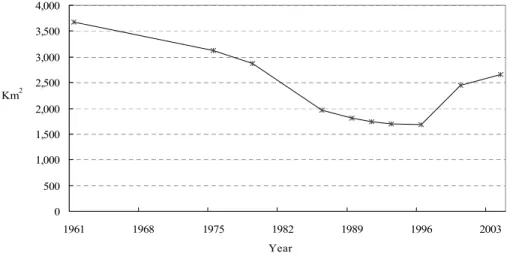
Figure 1. Habitats of mangrove in Thailand (23 provinces) Source: Aksornkoae and Tokrisna㧔2004㧕
0 500 1,000 1,500 2,000 2,500 3,000 3,500 4,000
1961 1968 1975 1982 1989 1996 2003
Year Km2
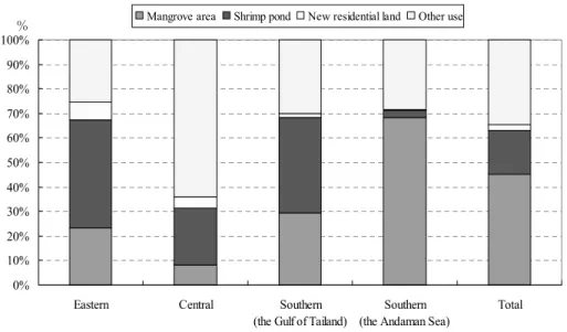
Figure 2. Changes of mangrove area in Thailand (23 provinces), 1961±2004
Note:These are generated by using the data from the below source.
Source: Geo-Informatics, National Park, Wildlife and Plant Conservation.
Rhizophoraceae family, which is characterized by salt tolerance, thick leaves, and many aerial roots. Mangrove forms an important ecosystem between the land and the sea area that is indispensable plant and animal habitat. Moreover, mangrove plays an important role in stabilizing shorelines by protecting coastal streams and estuaries against tidal wave and soil erosion. Mangrove in Thailand inhabits 23 provinces (6 provinces on the coast of the Andaman Sea and 17 provinces on the coast of the Gulf of Thailand), approximately half of the total 2614 km coastline of Thailand (Aksornkoae and Tokrisna, 2004) (see Figure 1).
Figure 2 shows changes in the area covered by mangrove in Thailand (23 provinces) from 1961 to 2004. Mangrove in Thailand has been steadily deforested from 1961 to 1996 and has been reduced to about half of the original area, from 3679 km
2in 1961 to 1685 km
2in 1996. After 1996, however, mangrove forestation began to increase and reached 2658 km
2in 2004, which is about 3/4 of the area covered by mangrove in 1961. In other words, in the 8 years between 1996 and 2004, mangrove forests recovered approximately half the loss experienced in previous years. In general, mangrove loss has been attributed to an increase in the demand for land as a result of population growth and economic development. The land converted from mangrove forest has been used for aquaculture (especially shrimp farming);
agriculture; mining (tin); salt production; urbanization; construction of houses, factories, roads, and ports; and power plants. Illegal cutting for household timber and fuel has also impacted mangrove loss. (Aksornkoae and Tokrisna, 2004)
Figure 3 shows mangrove deforestation and its conversions to other land uses from 1991
to 1996 (the mangrove area in 1961 is set to 100%). The five bar graphs represent four regions
in Thailand and the four-region total. These four regions are the Eastern region east of
0%
10%
20%
30%
40%
50%
60%
70%
80%
90%
100%
Eastern Central Southern
(the Gulf of Tailand)
Southern (the Andaman Sea)
Total 䋦 Mangrove area Shrimp pond New residential land Other use
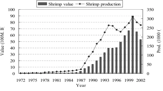
Figure 3. Mangrove deforestation and its conversions to the other land uses, 1991±1996
Note:The mangrove area in 1961 is set to 100%. These are generated by using the data from the below source.
Source: Geo-Informatics, National Park, Wildlife and Plant Conservation.
Bangkok (including 5 provinces); the Central region near Bangkok (including 6 provinces);
the Southern region on the coast of the Gulf of Thailand (including 6 provinces); and the Southern region on the coast of the Andaman Sea (including 6 provinces). Looking overall at the four regions, 55% of the total mangrove area in 1961 had been deforested and about 18%
(one third of destroyed mangrove area) converted into shrimp ponds by 1996. Another 2% of the mangrove area had been converted into new residential land and 35% converted for other uses.
The percentage of mangrove land converted into shrimp ponds is 44% in the Eastern region, 39% in the Southern region along the Gulf of Thailand, 23% in the Central region, and 2% in the Southern region along the Andaman Sea. Conversions into new residential land are very small² 7% in the Eastern region, 5% in the Central region, 2% in the Southern region along the Gulf of Thailand, and almost 0% in Southern region along the Andaman Sea.
Conversions into other uses are most common in the Central region near Bangkok at around 64%, which is two times higher than the other three regions. A possible explanation might be that the demand for land for economic development is higher in the Bangkok area than in other regions.
The previous section demonstrated that deforestation in Thailand accounted for a loss of
half of all mangrove forests during the 35 years from 1961 to 1996, and about one-third of the
destroyed area has been converted into shrimp ponds. How has the shrimp culture industry in
Thailand been developed during the same period? Figure 4 shows changes in the number of
0 5 10 15 20 25 30 35 40
1972 1975 1978 1981 1984 1987 1990 1993 1996 1999 2002 Year
Farms(1000farms)
0 10 20 30 40 50 60 70 80 90
Area(1000Km2)
Shrimp farm Culture area
Figure 4. Changes of the number of shrimp farms and culture area in Thailand, 1972 - 2002
Note:These are generated by using the data from the below source.
Source: Statistics of Shrimp Culture, Department of Fisheries, Ministry of Agriculture and Cooperatives.
shrimp farms and culture areas in Thailand between 1972 and 2002. Both graphs clearly show a steady rise in the development of the shrimp culture industry in Thailand during this period.
It is helpful to examine the historical background of shrimp farming in Thailand.
3In its early stages, shrimp production in Thailand was a by-product of salt production; wild shrimp strayed into the salt pans and were harvested. Subsequently, farmers stocked intentionally captured natural larvae in brackish ponds (a mixture of seawater and fresh water), then KDUYHVWHG WKHP DIWHU WKH JURZWK 7KLV VKULPS FXOWXUH PHWKRG LV FDOOHG ³H[WHQVLYH shrimp farming
4.´ Most brackish water ponds were usually converted from or were part of a salt pan.
During this early period, the species raised were banana shrimp (Peneaus merguiensis) and school shrimp (Metapenaeus sp), which depended on natural larvae and fed on wild seaweed and plankton.
In the late 1960s, the number of shrimp farms started to increase gradually as rising shrimp prices made shrimp farming more profitable than salt production. Shrimp ponds were constructed on the coastline and the banks of canals by clearing mangrove trees and taking advantage of the natural tide system for water exchange. The success of artificial incubation for banana shrimp and black tiger shrimp (Peneaus monodon) in 1973 accelerated the increase
3The history of shrimp culture in Thailand in this section is attributed to Aksornkoae and Tokrisna (2004).
4According to the census, extensive shrimp farming is defined as a culture method that uses only natural larvae and feeds in pond water that is derived from canals (Taya, 2003). The culture ponds used are relatively large, approximately 20-30 ha per pond. It takes 45-90 days for this method to raise shrimps, so the cost is low but the productivity is also low. In the semi-intensive shrimp farming method, farmers stock the larvae from the hatcheries (less than 24,000 fries per 1 rai (= 1600 m2) of a pond), use artificial feed, and manage pond water by pumping from canals to improve the productivity. This culture system fits in between the extensive and intensive systems (a fuller explanation appears later).
0 10 20 30 40 50 60 70 80 90 100
1972 1975 1978 1981 1984 1987 1990 1993 1996 1999 2002 Year
Value(100M.B)
0 50 100 150 200 250 300 350
Prod.(1000t)
Shrimp value Shrimp production
Figure 5. Changes of shrimp production and value in Thailand, 1972 - 2002
Note:These are generated by using the data from the below source.
Source:Statistics of Shrimp Culture, Department of Fisheries, Ministry of Agriculture and Cooperatives.
in shrimp farms. The number of shrimp farms gradually increased from 1972 to 1987, but after 1988 to 2000 they increased more rapidly due to the introduction of a new shrimp species, the black tiger shrimp, which had a higher profit rate because of its higher tolerance and better survival rate. In 1983, a multinational company from Taiwan started a joint venture with local investors, which used black tiger shrimp in an ³intensive shrimp farming
5´ system. The development of this new technology caused a rapid increase in the number of shrimp farms after 1988.
In 1991, the Thai government enforced a new law (Cabinet Resolution) that prohibited the conversion of conserved and fertile mangrove areas into shrimp ponds, which slowed down the increase in shrimp farms temporarily during 1992 and 1993. Under this law, it became impossible to construct new shrimp ponds in the coastal area. However, investment in intensive shrimp farming continued to steadily increase since it did not require large shrimp ponds, which caused a rapid increase in the total number of shrimp farms from 1988 to 2000 (although there was a temporary decline because of the Asian economic crisis in 1997). This increase depended on the success of black tiger shrimp hatcheries, of course; at the same time,
5This culture system uses a small pond, such as a rice field, in which shrimp is cultured by high larvae density and artificial mixed feed. To protect against disease infection, the farmers manage water quality by adding antibiotics and chemical products such as nutrients for 24 hours. Moreover, the farmers settle paddle wheel machines in shrimp ponds to maintain oxygen in the water, which is consumed during the decomposition of wastes from shrimp and artificial feeds. The culture ponds are small-sized, 0.5-1 ha per pond. According to the census, intensive shrimp farming is defined as a culture method that stocks more than 24,000 larvae per 1 rai, feeds 3-5 times per day, settles 1 paddle wheel per 1-2 rai of a pond, and takes 4-5 months for growth (Taya, 2003).
it was supported by the development of the shrimp feed industry, the technique of intensive shrimp farming, and the high shrimp price in the international market.
In more recent years (2001 and 2002), the number of shrimp farms decreased sharply.
According to our field studies in Thailand, this was due to falling shrimp prices in the international market, possibly caused in part by an increase in shrimp production in other countries ( such as Indonesia, Vietnam, and India ). Indeed, even in the U.S., the largest importer of shrimp from Thailand, shrimp imports from Ecuador have increased gradually.
Moreover, Thai shrimp farmers are confronted with the problems of infectious disease and lack of parental shrimps.
Another graph in Figure 4 shows changes in the shrimp culture area in Thailand from 1972 to 2002. The shrimp culture area, as well as the number of shrimp farms, showed an upward trend from 1972 to 1991. During the period between 1992 and 2000, however, the size of the shrimp culture area became stable. This was due to the Cabinet Resolution prohibiting the conversion of conserved and fertile mangrove areas into shrimp ponds; it also reflected the shift from extensive to intensive shrimp farming techniques. Intensive shrimp farming did not require the large shrimp ponds; therefore, this shift in the shrimp culture method gradually decreased mangrove deforestation.
6Shrimp culture areas declined by 5% in 2001 and 16% in 2002, due to the shift in shrimp culture techniques.
Figure 5 shows changes in shrimp production (line graph) and value (bar graph) in Thailand from 1972 to 2002. Both graphs show an upward trend, similar to what the graphs in Figure 4 show for the number of shrimp farms and area. Production and value increased gradually until 1987, then experienced a rapid increase from 1988 to 1994, which is partially attributable to the impact of black tiger intensive shrimp farming beginning in 1983. From 1995 to 1997, shrimp production slowed down due to widespread shrimp infectious disease caused by the deterioration of water quality and nourishment. After 1998, the shrimp disease problems were solved and shrimp production increased again. The steady and rapid increase in shrimp value from 1988 to 2000 is due to the stability of the international market price of shrimp and the Japanese shrimp demand (Traesupap et al., 1999). Both shrimp production and value decreased in 2001 and 2002, which was caused by a decline in the international market price of shrimp.
3. Empirical model and hypothesis test
To analyze the EKC relationship between mangrove deforestation and income level, the empirical mode in this study uses the quadratic reduced form, which has been used for
6In the1990s, the expansion of the culture area stabilized because of the shift to intensive shrimp farming and the GHYHORSPHQWRIDQHZFXOWXUHV\VWHPFDOOHGD³FORVHGVKULPSIDUPLQJV\VWHP´,QWKLVV\VWHP, once the water is poured into the shrimp ponds, it almost needs no exchange. The farmers monitor the water condition and maintain a constant salt concentration. The water in the pond is imported from the sea by truck and it is carefully inspected before being poured into the pond. This system rapidly spread in the Central region near Bangkok starting around 1996, so that shrimp ponds have been constructed not only in the coastal areas but also in agricultural land in inland areas. In November 1998, however, the National Environment Board banned shrimp farming in freshwater areas (particularly in the Central region) out of concern about land chlorination and environmental degradation because too many agricultural lands were converted into ponds.
empirical EKC studies in general.
7This model includes per capita gross provincial production (GPP) and its square term to test the EKC hypothesis. Previous EKC studies for deforestation examined the reason why the EKC relationship exists and showed important determinants of EKC, such as population growth rate, population density, price of products, structural factors, political factors, and institutional factors. Hence this study adds the important determinants of mangrove deforestation --increasing population pressure (population growth rate and population density) and industrial structural change on the economy (industrial share)-- to the empirical model.
Population growth pressure indicates rising land demand, which is the main cause of deforestation, so it is always included in the empirical model. Population density data at the provincial level, however, is not available, so only the population growth rate is included as an explanatory variable in the model. Moreover, as a structural variable, the GPP share of the shrimp industry has a strong relationship to mangrove deforestation and is therefore included as one of explanatory variables in the model.
Industrial share affects the EKC relationship between mangrove deforestation and income level as follows. In the early stages of economic development, mangrove forests are intact. However, as the economy begins to change structurally, agriculture and fisheries shift to aquaculture and manufacturing. During this stage, both economic development and mangrove deforestation are underway. As the economy continues to develop and moves into the second structural change, those industries shift again to the service and informational and technological industries. In this stage, society can afford to pay attention to environmental degradation, and environmental protection laws are enforced and reforestation projects begun, which finally reduces mangrove loss.
The empirical model in this study is represented by the following equation:
M 㧰it Į
iȕ
1Y
itȕ
2(Y
it)
2ȕ
3ǻ<itȕ
4P
itȕ
5S
itȕ
6D
itİ
it, (1)
where, i 㧔 «n㧕 is each province (23 provinces) and t is each year. Hence, M 㧰itindicates a mangrove deforestation index for i-th province in t-th year. In this study, as a mangrove GHIRUHVWDWLRQLQGH[ERWKµDQQXDOPDQJURYHGHIRUHVWDWLRQ¶DQGµWRWDOPDQJURYHGHIRUHVWDWLRQ
(used by Shafik and Bandyopadhyay, 1992) are utilized. The former is the yearly change in mangrove area and the latter is the change in mangrove area between the earliest date, 1975, and latest date.
Y
itis the Gross Provincial Product (GPP) per capita for i-th province in year t. (Y
it)
2is its square values;
ǻ<itrepresents average GPP growth rate for i-th province in year t; P
itis Population Growth Rate for i-th province in year t; S
itis Shrimp Value Share for i-th province in year t; and D
itis dummy for the shock from the Asian Economic Crisis in 1997 and 98 (1 in WKH &ULVLV \HDU RWKHUZLVH ]HUR 0RUHRYHU Į
iis an intercept term that reflects technical innovation and cultural and social structure in i-th province; ȕ¶s are coefficients for each
7Although a log-quadratic model has been utilized in many empirical studies of the EKC relationship to deforestation, we could not use it because the mangrove deforestation index included some minus values.
variables; and ݶs are disturbance terms.
As a pooled regression, the empirical model can be estimated using three different estimation techniques: the one point fixed model, the fixed effect model, and the random effect model. In the preliminary estimation, the no effect model was significantly rejected in favor of the fixed effect model using the F test, and the random effect model was significantly rejected in favor of the fixed effect model using the Hausman test. Therefore, in this estimation, the fixed effect model is employed.
8The fixed effect model is also referred to as the least squares dummy variable (LSDV) model, which has a cross section group-specific constant term in the estimation model. Since the pooled data used in this study was collected from 23 different provinces, there should be included some province-specific historical and structural differences. Therefore, the use of the fixed effect model is a reasonable choice here.
If the pooled data used in this model has different sizes according to each province size, the existence of a heteroscedasticity problem can be suspected. Hence, in the preliminary estimation, we also conducted the Wald test, after which the null hypothesis of homescedasticity was significantly rejected as predicted (there exists heteroscedasticity). To correct this problem, the weighted least square (WLS) approach is utilized in general. This technique transforms the variance of observation to give larger weight to observation with small variance. In this estimation, the two-stage feasible generalized least square (FGLS) technique is employed since only the cross section weight is considered.
On the other hand, since the pooled data used includes time-series data, the autocorrelation (AR) problem should be examined by using the Durbin-Watson (DW) statistic.
If the null hypothesis (no autocorrelation) is rejected, the AR term should be included in the model to correct the autocorrelation. In that case, the iterated feasible generalized least square (iterated FGLS) approach is utilized for the estimation; however, care should be taken not to lose too many degrees of freedom in the estimation. While the effects of all combinations of the explanatory variables on mangrove deforestation are estimated by using the estimation model (1), at the same time, the EKC relationship between mangrove deforestation and income level is determined. To show the existence of the EKC hypothesis, the null hypothesis of both zero coefficients RI ȕ
1DQG ȕ
2ȕ
1= ȕ
2= 0) should be rejected and the alternative K\SRWKHVLV ȕ
1> DQG ȕ
2< 0) accepted. If this alternative hypothesis is satisfied and demonstrates the evidence for the existence of EKC, it is useful to estimate an EKC turning point, which indicates the income level at which mangrove deforestation begins to decline.
The EKC turning point can be calculated by dividing estimated coefficient, ȕ
1by -ȕ
2. 7KHVLJQIRUWKHHVWLPDWHGFRHIILFLHQWRIWKH*33JURZWKUDWHȕ
3is unpredictable since it is situational. For example, if mangrove only plays an input role on the production process in Thailand, the increase in the GPP growth rate accelerates mangrove deforestation. However, if the GPP grows and the technology develops and mangrove is no longer necessary for inputs, then the increase on the GPP growth rate reduces mangrove loss. The sign for the estimated coefficient oISRSXODWLRQJURZWKUDWHȕ
4is expected to be positive, because the rising pressure
8See Chapter 13 in Greene (2003).
on population growth causes the increase in land demand, which quickens mangrove deforestation.
It is also difficult to predict the sign for the estimated coefficient of the industrial share on VKULPSIDUPLQJȕ
5. In general, the development of the shrimp farming industry accelerates mangrove deforestation, but that is the case for extensive shrimp farming. As mentioned in section 2, shrimp farming has shifted from extensive to intensive shrimp farming techniques, which reduces mangrove deforestation. Therefore, the expected sign for the shrimp industrial share depends on the difference in shrimp value between the two culture techniques. Finally, the sign for the estimated coefficient of dummy vDULDEOH ȕ
6is expected as minus. An economic shock always decreases the production level in an economy, thereby working to reduce environmental degradation.
4. Data
This analysis uses pooled data on mangrove areas that combine cross sections on 23 provinces in Thailand and a time series of 10 years (1961, 75, 79, 86, 89, 91, 93, 96, 2000, and 2004). The data on mangrove areas, except for 1961 data, are very accurate since they are derived from a Landsat-5 (TM) satellite. Unfortunately, for 1961, data on 6 provinces are missing and data for the Eastern and Central areas are also extremely small values compared to 1975. Therefore, we suspect measurement errors or differences in methodology in 1961, and have removed the 1961 data from the analysis.
From the data on mangrove areas, we created 2 types of indexes, a "total mangrove GHIRUHVWDWLRQ´LQGH[DQGDQ³DQQXDOPDQJURYHGHIRUHVWDWLRQ´LQGH[ZKLFKLQGLFDWHWKHOHYHO of mangrove deforestation (the terms were first used by Shafik and Bandyopadhyay (1992))
9. The former index is the change rate of mangrove areas between the base year of 1975 and other years (the unit is %), which is available for 22 provinces except Bangkok since its data in 1975 is zero. The latter index is the change of mangrove areas between years (the unit is square Km), which is available for all 23 provinces. Therefore, each index has 8 data points in the time series, so that the available observation numbers are 176 for the total mangrove deforestation index and 184 for the annual mangrove deforestation index.
The Gross Provincial Product (GPP) expresses the provincial level of Gross Domestic Product (GDP). Because the early studies of EKC used the 1985 US$ basis, we did the same, by converting the nominal GPP into the real GPP by using a GDP deflator with the 1985 US$ basis (= 100). This allows us to compare our results with the early studies and possibly avoid some autocorrelation problems in the time series data. In our analysis, the GPP per
97KHµWRWDOPDQJURYHGHIRUHVWDWLRQ¶LQGH[LVFDOFXODWHGE\GLYLGLQJWKHGLIIHUHQFHEHWZHHQWKHPDQJURYHDUHDLQWKHEDVH year of 1975 (Mi,75) and the one in yeart(Mi,t) by the one in 1975 (Mi,75) ; and multiplying 100;
MLi,t=
75 ,
, 75
, ) 100
( i
t i i
M M
M u
, (i «SURYLQFHVH[FHSW%DQJNRN
7KHµDQQXDOPDQJURYHGHIRUHVWDWLRQ¶LQGH[LVVLPSO\FDOFXODWHGE\H[WUDFWLQJWKHPDQJURYHDUHDLQ\HDUt-1 (Mi,t-1) from the one in yeart(Mi,t);
MLi,t=Mi,t㧙Mi,t-1, (i «SURYLQFHV
capita is used, so each GPP is divided by the population in each province. Moreover, the GPP growth rate is not the per capita level but the per province level.
$VPHQWLRQHGLQ6HFWLRQWKHGDWDIRU7KDLODQG¶VWRWDOQXPEHURIVKULPSIDUPVFXOWXUH area, shrimp production, and shrimp value are available from 1972 to 2002. The data on the provincial level, however, are limited from 1976 to 2002. Since the provincial data for mangrove area, GPP, and population are available from 1975 to 2004, we utilized the data for shrimp production in 1976 and 2002 as proxies for 1975 and 2004, respectively. The industrial share of shrimp farming to total GPP is calculated by dividing the shrimp production in each province by the GPP in each province (1985 US $ level). There are many zero level of shrimp production and value in the early years of the data; in those cases, however, the zeros were kept intact and used for the estimation.
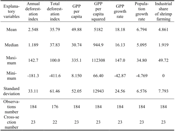
Finally, the sources of the data are listed in Table A1 in the Appendix. The statistics for all data are also shown in Table A2 in the Appendix. We can see there is a wide variance in the data from the table. The size of the data indeed depends on the situation in each province. The average of GPP data is 49880 Thailand Baht, which is converted into US$1833 (1985 US
$ level).
5. Empirical Results
7DEOHVKRZVWKHHVWLPDWLRQUHVXOWVRIWKHUHJUHVVLRQHTXDWLRQLQWKHFDVHRIPRGHO
Table 1 shows the estimation results of the regression equation (1) in the case of model I, which uses total shrimp industrial share. The left-hand column presents the estimation results using the total mangrove deforestation index as an explained variable (Case 1); the right-hand column presents results based on the annual mangrove deforestation index as an explained variable (Case 2). In the preliminary estimation for case 1, Durbin-Watson (DW) statistics shows 1.350 (< d
l= 1.57), which indicates the existence of a positive autocorrelation problem.
We added the AR (1) term in the fixed effect model to correct the problem; however, we could not estimate the model because of the singular variance-covariance matrix. Therefore, we used the no effect model with the AR(1) and AR(2) terms by using iterated feasible weighted least square (FGLS) in model I.
In case 1, the number of cross sections in the data is 22, because the Bangkok province is excluded as mentioned in previous section. The time series data includes 8 years, from 1979 to 2004, so that the number of total observations is 176, but the degrees of freedom reduced to 132 by correcting autocorrelation. The Adjusted R
2is 0.916, which indicates the high explanatory power of the model. The F-value is also very high at 179.9. After correcting autocorrelation, the DW statistics are 1.887 (> d
u= 1.78), in which the null hypothesis of no
DXWRFRUUHODWLRQȡ ZDVQRWUHMHFWHGIn case 1, the estimated coefficient for the GPP per capita has the expected positive sign
ȕ
1> 0) and is statistically significant at the 1% confidence level. The estimated coefficient
for the GPP per capLWD VTXDUHG KDV WKH H[SHFWHG QHJDWLYH VLJQ ȕ
2< 0) and is statistically
significant at the 5% confidence level. These results strongly suggest the existence of the
Table 1. Estimates for Model I
(Explanatory variables) Case 1
(Total deforestation index㧕
Case 2
(Annual deforestation index)
Constants
㧙20.65 㧙6.502
(23.75) (5.062)
GPP per capita 0.481 0.172
(0.179)*** (0.083)**
GPP per capita squared
㧙0.0010 㧙0.00049
(0.0005)** (0.00021)**
GPP growth rate
㧙0.069 㧙0.087
(0.036)* (0.055)
Population growth rate 0.304 1.535
(0.189) (0.411)***
Industry share of 0.040
㧙0.435
shrimp farming (0.189) (0.460)
Dummy
㧙9.050 㧙29.93
for Asian Economic Crisis (2.249)*** (7.699)***
AdjustedR2 0.916 0.410
DW 1.887 2.130
F-value㧔P-value㧕 179.9 (0.000) 5.538 (0.000)
The number of cross-section 22 23
The number of time series 8 (1979-2004) 8 (1979-2004)
Observations
㧔with AR㧕
176 (132) 184EKC turning point (1985US㧐㧕 $8451 $6505
Estimation model No effect + AR + WLS Fixed effect + WLS Note1: Standard errors are in parentheses.
Note2: *,**, and***are statistically significant at 10, 5, and 1 % significance level.
Note3:EKC turning points are calculated by using international exchange rate (US$1 = 27.21THB).
EKC hypothesis. The estimated coefficient for the GPP growth rate shows negative sign and is statistically significant at the 10% confidence level, which means that the increase of GPP growth reduces mangrove deforestation. Moreover, the estimated coefficient for the population growth rate has the expected positive sign, but it is not satisfied with the 10% level of significance (it is 11% of significance, however). This weakly suggests that the rising of the population growth rate accelerates mangrove deforestation.
On the other hand, in the preliminary estimation of case 2, using the DW test, the null
hypothesis is not rejected (DW statistics are 2.130 < 4-d
u= 2.22), making it unnecessary to
correct autocorrelation. Hence, in case 2 the fixed effect model is estimated by two-step
FGLS. The number of cross sections in the data is 23, all of which are provinces possessing
mangrove. The number of observations is 184, and all were gathered from a time series of 8
years, from 1979 to 2004. However, the adjusted R
2is 0.410, which indicates a lower
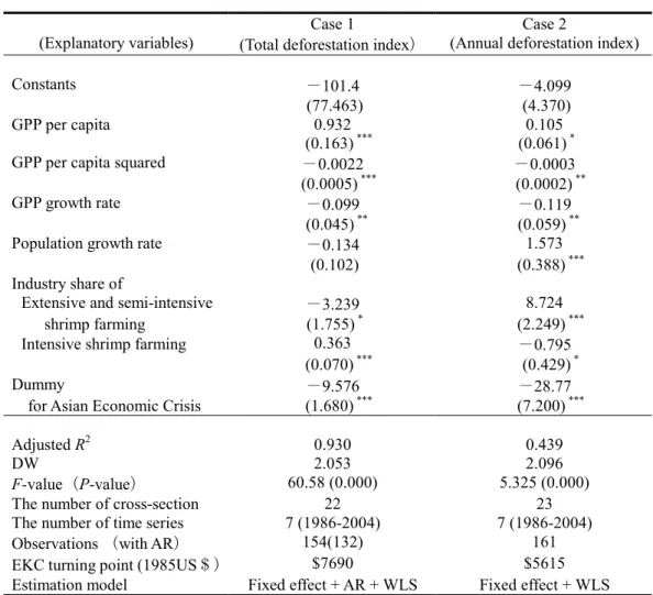
Table 2. Estimates for Model II
(Explanatory variables) Case 1
(Total deforestation index㧕
Case 2
(Annual deforestation index)
Constants
㧙101.4 㧙4.099
(77.463) (4.370)
GPP per capita 0.932 0.105
(0.163)*** (0.061)*
GPP per capita squared
㧙0.0022 㧙0.0003
(0.0005)*** (0.0002)**
GPP growth rate
㧙0.099 㧙0.119
(0.045)** (0.059)**
Population growth rate
㧙0.134
1.573(0.102) (0.388)***
Industry share of
Extensive and semi-intensive
㧙3.239
8.724shrimp farming (1.755)* (2.249)***
Intensive shrimp farming 0.363
㧙0.795
(0.070)*** (0.429)*
Dummy
㧙9.576 㧙28.77
for Asian Economic Crisis (1.680)*** (7.200)***
AdjustedR2 0.930 0.439
DW 2.053 2.096
F-value㧔P-value㧕 60.58 (0.000) 5.325 (0.000)
The number of cross-section 22 23
The number of time series 7 (1986-2004) 7 (1986-2004)
Observations
㧔with AR㧕
154(132) 161EKC turning point (1985US㧐㧕 $7690 $5615
Estimation model Fixed effect + AR + WLS Fixed effect + WLS Note1: Standard errors are in parentheses.
Note2: *,**, and***are statistically significant at 10, 5, and 1 % significance level.
Note3:EKC turning points are calculated by using international exchange rate (US$1 = 27.21THB).
explanatory power of the model than in case 1, and the F-value reduces from 179.9 to 5.538.
In the estimation results in case 2, the estimated coefficients for the GPP per capita and
the GPP per capita squaUHGKDYHWKHH[SHFWHGVLJQVȕ
1!DQGȕ
2< 0) and are both statistically
significant at the 5% confidence level. These results, like the case 1 results, strongly suggest
the existence of the EKC hypothesis. The estimated coefficient for the GPP growth rate also
shows a negative sign but is not statistically significant. Hence, in case 2 we cannot reach a
conclusion about the relationship between GPP growth rate and the EKC. The estimated
coefficient for the population growth rate has the expected positive sign, as in case 1, and is
statistically significant at the 1% confidence level. This strongly suggests that the increase in
the population growth rate accelerates mangrove deforestation.
The estimated coefficients for the industrial share of shrimp farming have a positive sign in case 1 and a negative sign in case 2, neither of which are statistically significant. These signs depend on how many shares based on data from extensive or intensive shrimp farming, as mentioned in section 3. The industrial share from extensive farming accelerates mangrove deforestation but the industrial share from intensive farming reduces mangrove destruction.
Since the industrial share results here are derived from a combination of these two farming methods, we cannot conclude anything statistically. Therefore, we analyze model II by dividing all industrial shares into categories of extensive or intensive shrimp farms.
Table 2 presents the estimation results for model II, which includes two parts of the industrial share of the extensive and intensive shrimp farms (the semi-intensive shrimp farming is included in the share of the extensive shrimp farm since the size of their shrimp ponds is very similar). In the same way as model I, the total mangrove deforestation index is used as an explained variable in case 1 and the annual mangrove deforestation index is employed as an explained variable in case 2. Since the data for the extensive and intensive shrimp farming are only available from 1987 to 2002, we used the data for 1987 and 2002 as proxies for 1986 and 2004, respectively. Therefore, the number of observations is 154 in case 1 and 161 in case 2.
In case 1 of the model II, the preliminary estimation shows DW statistics of 1.368 (< d
l= 1.57), which indicates positive autocorrelation, so we corrected the problem by adding an AR(1) term in the model (after correction, DW statistics are 2.053). Hence, in case 1 the fixed effect model is estimated by using iterated FGLS with an AR(1) term. The estimation results in case 1 show that the adjusted R
2is 0.930, which indicates a high explanatory power of the model; the F -value is also very high at 60.58. The estimated coefficient for the GPP per capita and the GPP squared both have the expected signs and both are statistically significant at the 1% confidence level. Hence, the results in case 1 also suggest the existence of the EKC hypothesis in model II. The estimated coefficient for the GPP growth rate shows a negative sign like model I and is statistically significant at the 5% confidence level. However, the estimated coefficient for the population growth rate has a negative sign, which is the inverse sign in model I and is not statistically significant.
In case 2, there is no autocorrelation problem in the preliminary estimation; therefore, we
estimated the fixed effect model by using the two-step FGLS. The time series data includes 7
years between 1986 and 2004 and the number of observations is 161. The adjusted R
2is
0.439, which indicates a lower explanatory power of the model than in case 1 and the F -value
is also smaller than in case 1. The estimated coefficient for the GPP per capita and the GPP
squared both have the expected signs as well as in case 2 in model I and are statistically
significant at the 5 and 10% confidence level, respectively. Hence, the EKC hypothesis is
satisfied in case 2. The estimated coefficient for the GPP growth rate shows a negative sign
and is statistically significant at the 10% confidence level (it is not statistically significant in
case 2 in model II). The estimated coefficient for the population growth rate has the expected
positive sign and is statistically significant at the 1% confidence level.
The estimated coefficient for the industrial shares in case 1 has the opposite sign from the one in case 2, but they are both statistically significant. In case 1, the estimated coefficients for the industrial share of both the extensive and semi-intensive shrimp farming and the intensive shrimp farming do not have the expected signs, but they are statistically significant at the 10% and 1% confidence level, respectively. In case 2, however, both industrial shares have the expected signs; the former is statistically significant at the 1% confidence level and the latter at the 10% confidence level. Therefore, the results strongly suggest that extensive and semi-intensive shrimp farming accelerate mangrove deforestation and intensive shrimp farming reduces mangrove destruction in case 2.
6. Discussion
First of all, we examined the existence of the EKC hypothesis and an EKC turning point based on the estimation results. In both models I and II, the estimated coefficients for the GPP per capita and the GPP per capita squared were satisfied with the expected signs. Also, they were statistically significant at the 1% or 5% confidence level except the GPP per capita term in model II, which were significant at the 10% level. Therefore, we can conclude that our results provide strong evidence of the existence of an EKC relationship between mangrove deforestation and income level in Thailand. That is, mangrove deforestation in Thailand increases as the income level rises, but the forests begin to recover once income reaches a threshold level.
From the estimated coefficients RI ȕ
1DQG ȕ
2in model I, the EKC turning points are calculated as $8451 in case 1 and $6505 in case 2 (1985 US$ base). In model II, the EKC turning points are computed as $7690 in case 1 and $5615 in case 2 (1985 US$ base). The EKC turning point in case 1 (the total mangrove deforestation index is used) in both models I and II are very similar to the results of a study by Lopez and Galinato (2005), in which turning points were calculated between $7000 and $8000 in the case of deforestation in Brazil, Malaysia, and the Philippines.
On the other hand, the EKC turning points in case 2 (the annual mangrove deforestation index is used) in both models I and II are very close to those in the study by Barbier and Burgess (2001), which were computed as $6182 in the case of deforestation in Asia. The fact that our estimated EKC turning points are very close to previous estimates strengthens the evidence of the existence of the EKC hypothesis. There is a difference of about $2000 in the EKC turning points of the total mangrove deforestation index and the annual mangrove deforestation index. This is because the former index recovers more slowly than the latter index (the shape of the EKC in the former index is flatter than the latter index).
Although the minimum EKC turning point calculated was $5615 (in case 2 in model II),
it is impossible for mangrove loss to recover if the turning point is far from the present GPP
per capita in Thailand. If we calculate the GPP per capita in 23 provinces in Thailand from the
collected data, it is about $4000 (1985 US$ base) even in 2004. Hence, the EKC turning point
that is the starting point for mangrove loss recovery has not yet been reached in Thailand.
Based on the collected data, however, the annual mangrove deforestation indexes show minus values in 22 provinces out of 23 provinces in 2000, which indicates recovery of mangrove loss in Thailand has already begun.
Next, we examined the effects of the shrimp farming industry on mangrove deforestation in Thailand. When the total industrial share of shrimp farming as a whole was used in model I, we did not get any useful results at all. However, when we included two divided industrial shares by shrimp culture technology in model II, we did get useful results. In model II, the estimation results in case 2 are stable and robust compared to the ones in case 1, because the former results did not change much between models I and II but the latter results did.
Therefore the estimation results in case 2 are more reliable than the ones in case 1. This might be the case because the autocorrelation was corrected at the expense of losing many degrees of freedom in case 1, which was not necessary in case 2.
Hence, we examined the relationship between shrimp farming and mangrove deforestation based on case 2 only. From the estimation results, it was confirmed that the development of extensive and semi-intensive shrimp farming techniques accelerated mangrove deforestation (shifted EKC upward) and the development of intensive shrimp farming reduced mangrove loss. As stated in section 2, many mangrove forests were cut down to create ponds for shrimp farming in the early stages of extensive shrimp farming; however, it was no longer necessary to clear forest in the 1980s, when intensive shrimp farming started to develop. The results of this study provide evidence that the development of technology in shrimp culture contributes to the reduction of mangrove deforestation.
In addition, the results of the factor analysis for mangrove deforestation clearly demonstrate that the rise of the population growth rate accelerated mangrove deforestation by shifting the EKC upward. This result supports the viewpoint that the fundamental cause of mangrove deforestation is increased demand for land due to population growth. It is also clear that as the GPP growth rate increases, mangrove loss is reduced and the EKC shifts downward.
The faster the GPP growth, the higher the mangrove loss recovery.
Also worthy of mention are the estimation results of the dummy variable used for expressing the effect of the Asian Economic Crisis in 1997 and 1998 on mangrove deforestation. The estimated coefficients for the dummy variable have the expected negative signs and are statistically significant at the 1% confidence level in all cases in both models.
These results strongly suggest that the Asian Economic Crisis slowed down the economy in Thailand, which reduced mangrove loss. In the same way that Moomaw and Unruh (1997) demonstrated the relationship between the EKC hypothesis and the Oil Crisis in 1979, these results demonstrate that the Asian Economic Crisis in the 1990s had the effect of stabilizing mangrove deforestation.
While the existence of an EKC relationship between mangrove deforestation and income level is indicated, some caution should be used in interpreting the empirical results. It is impossible to generalize the EKC hypothesis from these results, as pointed out by Arrow et al.
³(FRQRPLF JURZWK LV QRW D SDQDFHD IRU HQYLURQPHQWDO TXDOLW\´ ,Q WKis study, we
examined mangrove deforestation in Thailand, where economic development had been far
ahead of other developing Asian countries. Hence, the EKC hypothesis confirmed in this study does not necessarily fit in Indonesia and Vietnam, which are facing the same problem of mangrove deforestation. Moreover, although mangrove trees recover relatively easily, it may take hundreds of years for primeval forests to recover, and it may be impossible for fishery resources to recover.
This study remains incomplete due mainly to lack of data. We need annual data on mangrove area and pre-1975 data for more precise analysis; we also need data on population density for each province, which is always used in EKC studies as the causing factor of deforestation. Moreover, to examine the causing factor of the EKC, we should not only include industrial share as an explanatory variable in the model, but also international trade values, political factors (policies for land use and investment for reforestation projects), and institutional factors (ownership and corruption). Indeed, the Thai government enforced a new law (Cabinet Resolution) that prohibited the conversion of mangrove areas into shrimp ponds in 1991 and 1998 and began the major project of reforestation. Another factor that deserves attention is the tendency of companies in Thailand to bribe government officials to break environmental protection laws. These analyses are left for future research.
References
Aksornkoae, S. and R. Tokrisna (2004³2YHUYLHZRf shrimp farming and mangrove loss in 7KDLODQG´,Q%DUELHU(%DQG66DWKLUDWKDLHGVShrimp Farming and Mangrove Loss in Thailand, Edward Elgar, pp.37-51.
Antle, J. M. and G. Heidebrink (1995 ³(QYLURQPHQW DQG 'HYHORSPHQW 7KHRU\ DQG International (YLGHQFH´ Economic Development and Cultural Change, Vol. 43(3) pp.603-625.
Arrow, K., B. Bolin, R. Costanza, P. Dasgupta, C. Folke, C. S. Holling, B. Jansson, S. Levin, .0DOHU&3HUULQJV'3LPHQWHO³(FRQRPLFJRZWKFDUU\LQJFDSDFLW\DQGWKe HQYLURQPHQW´Science, Vol.268(5210), pp.520-521.
%DUELHU(%DQG-&%XUJHVV³7KH(FRQRPLFVRI7URSLFDO'HIRUHVWDWLRQ´Journal of Economic Surveys, Vol.15(3), pp.423-421.
%KDWWDUDL0DQG0+DPPLJ³,QVWLWXWLRQVDQGWKH(QYLURQPental Kuzets Curve for 'HIRUHVWDWLRQ $ &URVVFRXQWU\ $QDO\VLV IRU /DWLQ $PHULFD $IULFD DQG $VLD´ World Development, Vol.29(6), pp.995-1010.
&URSSHU 0 DQG & *ULIILWKV ³7KH ,QWHUDFWLRQ RI 3RSXODWLRQ *URZWK DQG (QYLURQPHQWDO4XDOLW\´American Economic Review, Vol.84(2), pp.250-254.
Greene, W. G. (2003), Econometric Analysis, fifth edition, Prentice Hall, pp.283-303.
Koop, G. and L. Tole (1999), ³,VWKHUHDQ(QYLURQPHQWDO.X]QHWV&XUYHIRU'HIRUHVWDWLRQ"´
Journal of Development Economics, Vol.58(1), pp. 231-244.
.X]QHWV6³(FRQRPLF*URZWKDQG,QFRPH,QHTXDOLW\´American Economic Review, Vol.45(1), pp.l-28.
Lopez, R. and G. Galinato (2005), ³Deforestation and Forest-Induced Carbon Dioxide
Emissions in Tropical Countries: How Do Governance and Trade Openness Affect the Forest-,QFRPH 5HODWLRQVKLS"´ Journal of Environment and Development, Vol.14(1), pp.73-100.
0RRPDZ:5DQG*&8QUXK³$UH(QYLURQPHQWDO.X]QHWV&XUYHV0LVOHDGLQJ Us? The Case of CO
2(PLVVLRQV´Environment and Development Economics, Vol.2(4), pp.451-463.
3DQD\RWRX7³'HP\VWLI\LQJWKH(QYLURQPHQWDO.X]QHWV&XUYH7XUQLQJD%ODFN%R[
LQWRD3ROLF\7RRO´Environment and Development Economics, Vol.2(4), pp.465-484.
3DQD\RWRX7³(PSLULFDOWHVWVDQGpolicy analysis of environmental degradation at GLIIHUHQW VWDJHV RI HFRQRPLF GHYHORSPHQW´ :RUNLQJ 3DSHU :3 7HFKQRORJ\ DQG Employment Programme, ILO, Geneva.
Panayotou, T. and S. Sungsuwan (1994),³An econometric analysis of the causes of tropical defoUHVWDWLRQWKHFDVHRI1RUWKHDVW7KDLODQG´LQThe Causes of Tropical Deforestation, eds. K. Brown and D. W. Pearce, London: University College London Press.
6KDILN 1 D ³(FRQRPLF 'HYHORSPHQW DQG (QYLURQPHQWDO 4XDOLW\ DQ (FRQRPHWULF
$QDO\VLV´Oxford Economic Papers, Vol.46, pp.757-773.
6KDILN1E³0DFURHFRQRPLFFDXVHVRIGHIRUHVWDWLRQEDUNLQJXSWKHZURQJWUHH"´LQ The Causes of Tropical Deforestation, eds. K. Brown and D. W. Pearce, London:
University College London Press.
Shafik, N. and 6 %DQG\RSDGK\D\ ³(FRQRPLF *URZWK DQG (QYLURQPHQWDO 4XDOLW\
Time Series and Cross-FRXQWU\ (YLGHQFH´ %DFNJURXQG 3DSHU IRU WKH :RUOG Development Report 1992, WPS904, The World Bank, Washington DC.
Taya, K. (2003) Shrimp Farming and Trade in Asia, Ch. 4, Seizando (written in Japanese).
Traesupap, S., Y. Matsuda, and H. Shima (1999³$QHFRQRPHWULFHVWLPDWLRQRI-DSDQHVH VKULPSVXSSO\DQGGHPDQGGXULQJWKHV´Aquaculture Economics and Management, Vol.3(3), pp.215-221.
Walter, H. (1971), Ecology of Tropical and Subtropical Vegetation, Edinburgh, Oliver &
Boyd.
Appendix
Table A2. List of data sources
Data Source
Mangrove area
㧔23 provinces㧕
Geo-Informatics, National Park, Wildlife and Plant Conservation GPP
㧔23 provinces㧕
Office of the National Economic and Social Development Board, Office of the Prime Minister
GDP deflator Economic and Financial Statistics, Bank of Thailand International
exchange rate Bank of Thailand Population
㧔23 provinces㧕
Registration Division, Local Administration Department, Ministry of Interior
Shrimp value
㧔23 provinces㧕
Statistics of Shrimp Culture, Department of Fisheries, Ministry of Agriculture and Cooperatives
Table A2. Summary statistics for data Explana-
tory variables
Annual deforest-
ation index
Total deforest-
ation index
GPP per capita
GPP per capita squared
GPP growth
rate
Popula- tion growth
rate
Industrial share of shrimp
farming
Mean 2.548 35.79 49.88 5182 18.18 6.794 4.861
Median 1.189 37.83 30.74 944.9 16.13 5.095 1.919
Maxi-
mum 142.7 100.0 335.1 112308 147.0 34.80 49.72
Mini-
mum -181.3 -411.6 8.150 66.40 -42.87 -4.769 0
Standard
deviation 33.11 61.46 52.05 12943 24.56 6.576 7.793
Observa- tions
number 184 176 184 184 184 184 184
Cross-se ction
number 23 22 23 23 23 23 23