論文の本文（k524）

博士論文

Initiation mechanism of

earthquake triggered

landslides during rainfall by

considering soil dynamic

properties

FIKRI FARIS

平成 23 年度入学

島根大学大学院総合理工学研究科博士後期課程

マテリアル創成工学専攻

主指導教員: 汪 発武

平成 26 年 7 月 22 日受理

i

Abstract

An earthquake struck Padang Province, West Sumatra, Indonesia, at 17:16 on September

30, 2009. The earthquake had a moment magnitude of Mw 7.6, and triggered landslides in

Tandikat, Padang Pariaman Regency. The landslides occurred during rainfall, and originated on mountains mantled with loose pumice, taking many lives. The unfortunate combination of intensive rainfall and earthquake probably decreased slope stability. This study seeks to examine the initiation mechanism of earthquake-triggered landslides during rainfall, and to develop a new approach to predict pore pressure increase by assuming reciprocal relationships between strain, stiffness, and excess pore pressure.

Field investigations, laboratory work and numerical modelling were conducted in this study. Assessment of rainfall infiltration used the Green-Ampt infiltration method, utilising hydraulic parameters determined from the field investigations. In order to assess slope stability, the concept of stiffness degradation was used to predict pore pressure increase due to earthquake. This was achieved by developing an empirical formulation based on cyclic triaxial test results. A new procedure based on the “rigid block on quasi plastic layer” assumption was developed to assess dynamic slope stability landslides during heavy rainfall. Additionally, stochastic analysis was performed by utilizing random variables of soil parameters to derive the probability distribution of landslide hazard.

Results from cyclic triaxial test experiments showed that initial effective confining pressure and initial shear stress had considerable influence on increase in pore pressure. Slope stability analysis using a rigid block on a quasi-plastic layer assumption and actual earthquake acceleration suggests that landslide may have occurred due to pore pressure build-up. The factor of safety decreased rapidly before earthquake acceleration reached its peak. At

ii

that time, the energy of the earthquake had not reached its maximum, suggesting that similar failures are likely to occur on saturated sliding zones during smaller earthquakes. This suggestion was supported by result of stochastic analysis. The stochastic analysis of the Tandikat landslide confirms that smaller earthquakes could possibly trigger catastrophic landslides during rainfall. Smaller peak ground acceleration of ≈0.15g could result in a more than 50% chance of Rsv >0.75, while the analysis of dry condition yields a 30% chance of

catastrophic level of landslide hazard. This suggests that rainfall condition increases the probability of catastrophic landslide. The effect of peak ground acceleration larger than 0.30g to the probability of Rsv >0.75 is negligible in a particular event. The results suggest that peak

ground acceleration of ≈ 0.30g is considered as the critical magnitude of ground acceleration that would result in a nearly 100% probability of catastrophic level of landslide hazard in the area.

iii

Acknowledgements

The thesis entitled “Initiation mechanism of earthquake triggered landslides during rainfall by considering soil dynamic properties” is written in order to fulfill the partial requirement for doctoral degree in Departement of Geoscience, Interdisciplinary Graduate School of Science and Engineering, Shimane University, Japan.

I would like to thank the Ministry of Education, Culture, Sports, Science and Technology (MEXT), Japan for awarding me the Monbukagakusho scholarship to study in Japan.

I wish to express my gratitude to my supervisor, Professor Fawu Wang of Project Center of Natural Disaster Reduction, Shimane University, Japan, for his full supports and great efforts in helping me to achieve my academic degree independently.

I sincerely thank all the professors and staff of the Department of Geoscience, Shimane University, for their moral and academic support. I will not forget to thank Professor Barry Roser for his immense help in checking the first manuscript of my paper. I am also grateful to Dr. Ying-Hsin Wu for his profound help in checking the early draft of this thesis.

I would like to express my appreciation to my master degree supervisor Dr. T. Faisal Fathani and Professor Dwikorita Karnawati who fully supported me to getting chance to study in Japan.

I extends my sincere thank to all my colleagues in Disaster Prevention Engineering Research Laboratory, Shimane University, especially to my friends, Messrs. Yasuhiro Mitani,

iv

Tomokazu Sonoyama, Mitsuki Honda, Yohei Kuwada, Hufeng Yang, Austin O.

Chukwueloka and Đỗ Ngọc Hà, for their support and contributions to my research.

The last but not least, I am grateful to my family, especially my beloved parents and my sister, who always encourage me to finish my study, my wife, Nurul Hidayati, for her tremendous love and patience in supporting my work, my daughter, Fasqiya, whose smiles and laughs amuse me all the time.

v

Table of Contents

Abstract ... i

Acknowledgement ... iii

Table of Contents ... v

List of Tables ... viii

List of Figures ... ix

1 Introduction ... 1

1.1 Background ... 1

1.1.1 Geological setting ... 3

1.1.2 Seismicity and meteorology ... 7

1.2 Aim of research ... 11

1.3 Scope of works ... 11

1.4 Thesis outline ... 12

2 Literature review ... 14

2.1 Effect of rainfall on earthquake triggered landslide ... 14

2.2 Initiation mechanism of landslide in pumice deposits... 15

vi

3 Research methodology ... 18

3.1 Field investigation ... 18

3.2 Infiltration model ... 21

3.3 Laboratory test ... 22

3.4 Excess pore pressure model ... 28

3.5 Stochastic slope stability and landslide volume analysis ... 31

3.5.1 Introduction to stochastic analysis ... 31

3.5.2 Groundwater modelling ... 31

3.5.3 Slope stability analysis ... 36

3.5.4 Monte-Carlo simulation ... 39

4 Initiation mechanism of the Tandikat landslide ... 41

4.1 Result of static triaxial test ... 41

4.2 Typical result of cyclic triaxial test ... 42

4.3 Effect of initial effective confining pressure on reference cumulative shear strain ... 47

4.4 Effect of initial shear stress on reference cumulative shear strain ... 49

4.5 Effect of initial effective confining pressure on stiffness degradation ... 51

vii

4.7 Numerical analysis ... 54

4.7.1 Excess pore pressure model fitting ... 54

4.7.2 Rigid block on quasi-plastic layer and simulation procedure ... 55

4.7.3 Pore pressure simulation and slope stability analysis during actual earthquake ... 59

5 Stochastic analysis of the Tandikat landslide ... 62

6 Conclusions ... 68

References ... 71

viii

List of Tables

Table 3.1 Input parameters used in the Green-Ampt infiltration model 20 Table 3.2 Pumice sand properties obtained from in situ measurement and laboratory tests 24 Table 3.3 Summary of CTX tests conducted during this study 27 Table 5.1 Parameters used in stochastic analysis 63

ix

List of Figures

Fig. 1.1 Widespread development of the Tandikat landslide (AP 2009) 2

Fig. 1.2 Location of the earthquake epicenter and landslide area (modified from Google Map 2014)

3

Fig. 1.3 The studied landslide and sampling location (a) The approximate width (W) and length (L) of the landslide are 90 and 120 m, respectively; (b) Panoramic view of the landslide location; (c) Sampling location

5

Fig. 1.4 Simplified geology of the earthquake affected area (modified from Petersen et al. 2007)

6

Fig. 1.5 Stratigraphy of the Tandikat landslide area (a) Outcrop showing the distinctive layer of sandy clay overlain by pumice sand; (b) Water ponding on the sandy clay layer, illustrating the low permeability of this layer

6

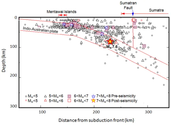
Fig. 1.6 Cross section of earthquakes location against subducting plate vs. depth and distance from subduction front (modified from Aydan 2009)

8

Fig.1.7 Earthquake accelerogram of M7.6 2009.09.30. (a) N-S direction; (b) Vertical direction

9

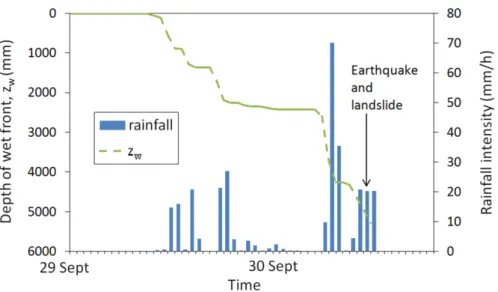
Fig. 1.8 Rainfall record in 40 hours prior to the earthquake in the Tandikat region 10

Fig. 3.1 Interpretation of landslide stratigraphy based on geological logging 20

Fig. 3.2 Infiltration analysis result showing depth of the wet front (zw) development

during the 40 hours before the earthquake

22

x

Fig. 3.4 Calculation scheme of strain, excess pore pressure and stiffness degradation 29

Fig. 3.5 Typical stress-strain loop of the cyclic triaxial test 30

Fig. 3.6 Scheme of groundwater model by rainfall infiltration 32

Fig. 3.7 Combined results of infiltration and groundwater model 35

Fig. 3.8 Scheme of slope stability analysis 38

Fig. 3.9 Flowchart of stochastic analysis to set specific volume ratio 40

Fig. 4.1 Effective stress path and transformed strength envelope of the static triaxial test 42

Fig. 4.2 Scheme of cyclic shear stress on a plane for a triaxial test specimen 43

Fig. 4.3 _{Time history of axial strain of cyclic loading triaxial test at}

0

σ′= 45 kPa 44

Fig. 4.4 _{Deviatoric stress-axial strain loop of cyclic loading triaxial test at}

0

σ′= 45 kPa 44

Fig. 4.5 _{Time histories of pore pressure ratio of cyclic loading triaxial test at}

0

σ′= 45 kPa 45

Fig. 4.6 Effective stress path (ESP) of mean effective confining pressure and shear stress at σ₀′= 45 kPa

45

Fig. 4.7 Excess pore water pressure ratio versus cumulative shear strain of cyclic loading triaxial test

46

Fig. 4.8 Excess pore water pressure versus cumulative shear strain for various initial effective confining pressures of cyclic loading triaxial test

48

Fig. 4.9 Reference cumulative shear strain vs. initial effective confining pressure of cyclic loading triaxial test

48

Fig. 4.10 _{Pore pressure ratio for}

0

σ′= 45 kPa versus cumulative shear strain with various shear stress ratios

xi

Fig. 4.11 _{Reference cumulative shear strain for}

0

σ′= 45 kPa and 90 kPa versus initial shear stress ratio

50

Fig. 4.12 _{Secant shear modulus versus cumulative shear strain for}

0

σ′= 45 kPa, 90 kPa and 135 kPa

52

Fig. 4.13 _{Secant shear modulus versus cumulative shear strain amplitude for}

0

σ′= 45 kPa with variable shear stress ratio

53

Fig. 4.14 _{Secant shear modulus versus cumulative shear strain for}

0

σ′= 90 kPa 53

Fig. 4.15 _{Secant shear modulus versus cumulative shear strain for}

0

σ′= 135 kPa 54

Fig. 4.16 Illustration of the rigid block on a quasi-plastic layer assumption 57

Fig. 4.17 Performance of the rigid block on quasi-plastic layer method on reference cumulative shear strain prediction at different confining pressures and initial shear stress ratios

58

Fig. 4.18 Model of ABAQUS 2D FEM and slope stability analysis points 59

Fig. 4.19 Time history of earthquake acceleration (EQ Acc), pore pressure ratio (ru), factor

of safety (Fs) considering ru (Fs with ru) and without considering ru (Fs w/o ru) at

the a. toe; b. middle; and c. crest

61

Fig. 5.1 Histogram of specific volume ratio (Rsv) in dry condition incorporated with

probability density and reversed cumulative curve

64

Fig. 5.2 Histogram of specific volume ratio (Rsv) during actual rainfall incorporated with

probability density and reversed cumulative curve

66

1

Chapter 1

Introduction

1.1 Background

Indonesia is an archipelagic country, which extends on one of the most active seismic areas in the world. In tectonic perspective, the west and south coasts of the archipelago take apart into Asian “ring of fire” that contains hundreds of active volcanic mountains, which extensively supplies loose volcanic materials. The tropical climate brings high precipitation in most part of the area. These facts make Indonesia highly vulnerable to geo-disasters triggered by the combined effect of earthquake and rainfall cycles. Whilst, possible occurrence of rainfall and earthquake at the same time is considerably small, the combination of both events may occur in seismically tropic areas, which inadvertently, could lead to severe live and property.

One of the most devastating earthquakes in Indonesian history struck Padang, West Sumatra Province at 17:16 on September 30, 2009. The earthquake had a moment magnitude

of Mw 7.6 (M7.6 2009.9.30) (USGS 2009), and caused over 1,000 deaths (EERI 2009). The

M7.6 2009.9.30 Padang earthquake triggered many landslides, and these accounted for more than 60% of the total death toll. The most extensive landslides occurred in Tandikat, Padang Pariaman Regency. These landslides buried hundreds of people, and flattened some villages (Fig. 1.1). A loose pumice ash layer on the mountains is thought to have been saturated by heavy rainfall before the earthquake. In this particular area, the probability of concurrent earthquake and rainfall events is high, since it has a tropical rainforest climate, and is also situated on a seismically active plate margin. Consequently, it is essential to study the

2

initiation mechanisms of landslides in saturated pumice sand, while considering the effects of the unfortunate combination of independent events such as heavy rainfalls and earthquakes.

3

Fig. 1.2 Location of the earthquake epicentre, mechanism and landslide area (modified from Google Map 2014)

1.1.1 Geological Setting

The Tandikat landslides occurred in Nagari Tandikat, Padang Pariaman Regency, around 60 km NNW of Padang City, West Sumatra Province, near the western coast of Sumatra, Indonesia (Fig. 1.2). This area experiences frequent high intensity earthquakes, due to the oblique movement of the Indo-Australia and Euro-Asian plates that formed the Sumatran Fault System. This also results in uplift of trench basement, which runs the length of the Barisan Mountains forming volcanic mountains parallel to the west coast (Aydan 2009).

Tandikat Padang 10 km Singkarak Lake Maninjau Lake Mt. Tandikat Epicenter of M7.6 2009.9.30 EQ

N

CMT Solution (NIED) Mt. Singgalang Mt. Marapi Mt. Talang

4

The landslides are located in a mountainous area around two volcanoes (Mt. Tandikat and Mt. Singgalang), and are extensively distributed on steep slopes inclined at 30 to 50 degrees. The slopes are mainly mantled by unconsolidated volcanic deposits that were transported from the nearby volcanic mountains. This topographical condition is considered to be an important contributory factor for landslides in Tandikat.

According to the Padang geological map (Petersen et al. 2007) in Fig. 1.4, landslide distribution was concentrated on Quaternary volcanic rock, denoted as Qvf (Quaternary volcanic rocks along flank of volcanoes). The surface deposits consist of silts, sands, and gravels, with remnants of pumice-tuff. Particularly in this area, impermeable clay strata are overlain by a porous pumice sand layer. From observations of landslide scarps and outcrops, the pumice sand deposits are clearly distinguishable from the clay strata (Fig. 1.5a). Measurements show the thickness of the pumice sand layers is generally about 2 to 3 meters. Low permeability of the clay layer was confirmed from water ponding which was observed on the exposed sliding surface of the clay layer (Fig. 1.5b). Sample of pumice sand was taken along 50 cm above the base of pumice sand deposit to nearly represent suspected sliding surface of the landslide (Fig. 1.3c).

5

Fig. 1.3 The studied landslide and sampling location. (a) The approximate width (W) and length (L) of the landslide are 90 and 120 m, respectively; (b) Panoramic view of the landslide location; (c) Sampling location

6

Fig. 1.4 Simplified geology map of the earthquake affected area (modified from Petersen et al. 2007)

Fig. 1.5 Stratigraphy of the Tandikat landslide area (a) Outcrop showing the distinctive layer of sandy clay overlain by pumice sand; (b) Water ponding on the sandy clay layer, illustrating the low permeability of this layer

7 1.1.2 Seismicity and meteorology

Several high magnitude earthquakes have been recorded in the subduction zone along

the west coast of Sumatra in the last few decades. The Mw 9.1 Aceh earthquake of December

26, 2004 caused the catastrophic Indian Ocean tsunami (USGS 2004). The Nias earthquake of March 28, 2005, and the South Sumatra earthquake of September 12, 2007, had

magnitudes of Mw 8.6 and Mw 8.5, respectively (USGS 2005; USGS 2007). The most recent

large earthquake was the September 30, 2009 Padang earthquake, which had a moment

magnitude of Mw 7.6. The epicenter was located offshore, WNW of Padang City, and the

hypocenter was located at a depth of 80 km, within the oceanic slab of the Indo-Australian plate (Fig. 1.6). The centroid moment tensor (CMT) solution taken from National Research Institute for Earth Science and Disaster Prevention (NIED) of Japan is shown in Fig. 1.2. From the CMT solution, the M7.6 2009.09.30 event was due to thrust faulting with slight dextral lateral slip. This earthquake has been interpreted as an indication of a higher possibility of an imminent mega-earthquake in this region (Aydan 2009). The M7.6 2009.09.30 earthquake accelerogram was provided by Meteorological and Geophysics Agency of Indonesia (BMKG). Figure 1.7 shows North-South (N-S) direction and vertical direction of M7.6 2009.09.30 earthquake acceleration. Unfortunately, West-East direction could not be provided due to some technical issue.

8

Fig. 1.6 Cross section of earthquakes location against subducting plate vs. depth and distance from subduction front (modified from Aydan 2009)

9

Fig. 1.7 Accelerogram of the M7.6 2009.09.30. (a) N-S direction; (b) Vertical direction (BMKG 2009)

One of the most damaged areas due to earthquake triggered landslide was in Cumanak Village of Nagari Tandikat, Patamuan sub-district, Padang Pariaman regency, about 60 km from the epicenter. Based on rainfall data interpreted from X-band Doppler Radar of the HARIMAU project provided by the Japan Agency for Marine-Earth Science and Technology (JAMSTEC) at Padang Pariaman Regency, rainfall of moderate intensity (about 70 mm/h) began at about 12:30, some hours prior to the earthquake shock at 17:16 local time on September 30, 2009 (Fig. 1.8). Antecedent rainfall of about 30 mm/h was recorded at the previous night. It is suspected that this rainfall played a major role in the triggering of the landslides. The contribution of rainfall to earthquake triggered landslides is of great concern in the volcanic area surrounding the west coast of Sumatra, which has equatorial weather that usually brings rainfall of high intensity, even during dry season periods (Sipayung et al.

10

2007). Based on the latest meteorological research on west coast of Sumatra, high intensity rainfall is frequently recorded in the late afternoon or evening, and distribution of such rainfall is strongly controlled by the mountainous topography of the area (Wu et al. 2009). The combined effects of seismic activity and meteorological conditions in this area create a high probability of failure of saturated volcanic deposits during earthquakes. These factors must be taken into consideration in geo-hazard assessment and risk management.

11

1.2 Aim of the research

The aim of this research is to study the initiation mechanism of earthquake triggered landslide during rainfall considering soil dynamic properties using deterministic and probabilistic approach. The specific objectives of this research are to:

1) Perform site investigation to gain more information about the geological features in specific areas, including rock/soil type and stratigraphy, geo-morphology, and the potential slip surface.

2) Examine the initiation mechanism of earthquake triggered landslides during rainfall, by developing an excess pore water pressure model using local pumice sand, and using a cyclic triaxial apparatus.

3) Perform combined groundwater model and geotechnical landslide analysis using appropriate computer code that may ultimately determine the probability of landslides during combined earthquake rainfall events in specific areas.

1.3 Scope of the works

The study site and sampling location of this research is located in Cumanak Village of Nagari Tandikat, Padang Pariaman Regency, West Sumatra Province, Indonesia (Fig. 1.3). This study focuses on the landslide event which occurred in the area due to earthquakes at 17:16 on September 30, 2009. The study supposed to contribute to research field of earthquake triggered landslide considering the effect of the rainfall through this particular case-based research.

12

This study examines the initiation mechanism of the landslide by developing an excess pore water pressure model of local pumice sand using cyclic triaxial apparatus and by performing numerical and slope stability analysis.

1.4 Thesis outline

This thesis presents a comprehensive study about the earthquake triggered landslide in Tandikat area, on September 30, 2009, to understand the nature of earthquake triggered landslide during rainfall. The main body of this thesis includes six chapters.

Chapter 1 gives information about the occurrence and the impact of landslide that triggered by September 30, 2009 Padang earthquake. This chapter shows the importance of the event to be considered and studied. This chapter provides information about geological condition, meterological condition, and seismicity of the region, which are important factors of the particular landslide event. The purposes and scopes of this work as well are mentioned in this chapter.

Chapter 2 consists of literature review of related research on earthquake triggered landslide and the effect of rainfall infiltration prior to landslide, the initiation mechanism of landslide on pumice deposits and stochastic slope stability analysis.

Chapter 3 includes the detailed explanation of research methodology fulfilled in this study. The detailed field investigation includes the technique for measuring soil hydraulic parameters using falling head permeameter test, and in situ density measurement. The description of infiltration model and its result are also mentioned. The detail about laboratory procedure, especially the detailed procedure of conducting cyclic triaxial test, including soil specimen preparations are explained in this chapter. The detail about the newly proposed

13

excess pore water pressure model, groundwater model and slope stability analysis for stochastic simulation are specified.

Chapter 4 includes the discussion about initiation mechanism of landslide which completely based on cyclic triaxial test results. This chapter discusses about cyclic triaxial test result, the excess pore water pressure model and its implementation to numerical analysis.

Chapter 5 discusses about the results of stochastic analysis of the Tandikat landslide using Monte-Carlo simulation.

14

Chapter 2

Literature review

2.1 Effect of rainfall on earthquake triggered landslide

Researches focusing on the effect of rainfall on earthquake triggered landslides are scarcely found in the literature. Sassa (2005) reported landslide disasters triggered by the 2004 Mid-Niigata Prefecture earthquake in Japan. The earthquake occurred 3 days after a heavy rainfall of Typhoon no. 23. The influence of rainfall on soil moisture prior to the earthquake was evaluated by Japan Meteorological Agency using hydrological model to obtain Soil Water Index (SWI) representing the amount of water stored under the ground surface. The landslides then were compared with those triggered by larger earthquake of the 1995 Hyogoken-Nambu earthquake during dry season. The 2004 Mid-Niigata earthquake triggered 362 landslides with a width more than 50 m and 12 large-scale landslides with volumes of more than 1 million cubic meters, while the only significant landslide triggered by the Hyogoken-Nambu earthquake was the 125 m wide Nikawa landslide with long travelling distance. This large difference was probably caused by the heavy rainfall prior to the Mid-Niigata earthquake. Based on this fact, Sassa (2005) emphasized that the combined effect of rainfall and earthquakes are necessary to be studied in landslide risk evaluation.

The study conducted by Chang et al. (2007) implemented the effect of rainfall on earthquake triggered landslide risk model. They used logistic regression to develop both

15

earthquake and typhoon triggered landslide risk models by considering a typhoon prior to the earthquake.

The initial mechanism of earthquake triggered landslide after rainfall was studied by Uzuoka et al. (2005). They performed site investigation, laboratory test and numerical simulation of Nishisaruta landslide triggered by July 26, 2003 Miyagi earthquake. They considered that high rainfall occurred 3 days before the earthquake was an important factor of the landslide. The rainfall was supposed to saturate the landslide mass before the earthquake and the main shock triggered the liquefaction of the sand fill in the slope which dramatically decreased the stability.

These researches confirmed the importance to consider the rainfall effect prior to earthquake. However, as far as we know, study about the effect of rainfall during earthquake is absence in the literature due to the exceptionality of the combined event of rainfall and earthquake.

2.2 Initiation mechanism of landslide in pumice deposits

Studies of initiation and post-failure mechanisms are conducted using different laboratory test methods. Studies of initiation mechanisms commonly use laboratory shearing tests considering “limited displacement” conditions (i.e. triaxial, hollow cylinder torsional shear, direct shear, and simple shear tests). Studies of post-failure mechanisms typically consider “large displacement” tests using ring shear tests.

The post-failure mechanism of volcanic deposits has been examined in several studies. A study of a long-travelled landslide in pyroclastic strata by Wang and Sassa (2000) used undrained ring shear apparatus to confirm grain crushing mechanism during shearing. Wang

16

et al. (2010) also evaluated the post-failure mechanism of long run-out pumice material from the Tandikat landslide, using the same apparatus.

Several studies have examined the initiation mechanism of landslides in common volcanic soils, and the role of pore water pressure build-up. Hyodd et al. (1998) examined the liquefaction characteristics of several crushable volcanic deposits. Suzuki and Yamamoto (2004) emphasized the liquefaction characteristics of the Shirasu pyroclastic deposit in Japan, using cyclic triaxial tests on disturbed and undisturbed samples. However, specific research on the dynamic properties of pumice sand and its relation to pore water pressure generation is rare.

Researches based on excess pore water pressure models mainly use regular sand for laboratory tests, with very limited effort focused on the dynamic behaviour of volcanic sand, especially pumice sand. Seed et al. (1976) and Lee and Albaisa (1974) used clean sand to study liquefaction, and to develop an excess pore water pressure model based on the number of cyclic loads. Yamazaki et al. (1985), Sugano and Yanagisawa (1992) and Jafarian et al. (2012) used Toyoura silica sand to derive excess pore water pressure models based on the strain energy concept, using a variety of laboratory tests. Work on the behaviour of pumice during dynamic loading has been reported by Marks et al. (1998) and Orense and Pender (2013). These authors studied the liquefaction characteristics and resistance of crushable pumice soils from North Island, New Zealand, based on undrained cyclic triaxial tests and field test data. They confirmed that pore pressure has been built up during shearing. Nevertheless, any empirical model for excess pore pressure generation in such material has not yet been developed.

17

2.3 Stochastic slope stability analysis

Determining stability of natural slope is a challenging task due to its complex nature and heterogeneity of the slope material. It also involves uncertainties in determining soil parameters and properties due to limited sampling and testing techniques (Griffiths et al. 2002). To deal with uncertainties in determining slope stability, stochastic approach involving random variables was used.

The probabilistic analyses were widely used in geotechnical field to deal with significant uncertainties in association with slope stability problem (Chowdury and Xu 1994). Many researches implemented probabilistic approach by using Monte-Carlo procedure to consider uncertainty in assessing earthquake triggered landslide, e.g. Wang et al. (2008), Refice and Capolongo (2002), and Shou and Wang (2003). Likewise, this study used Monte-Carlo simulation to consider uncertainty of soil parameters in obtaining probability of landslide hazard.

18

Chapter 3

Research methodology

3.1 Field Investigation

Field investigations were conducted to understand the geological features in the area and the mechanism of the landslides. Methods included outcrop observations, soil sampling, and subsurface examination using boreholes. The interpretation of landslide stratigraphy based on geological logging is presented in Fig. 3.1. The bedrock comprises moderately weathered medium- to fine-grained andesitic sandstones, which are overlain by stiff sandy clay, followed by unconsolidated tuffaceous pumice sand. The tuffaceous pumice sand forms the main material of the landslide body.

The low density and high porosity of the pumice sand in its original state was confirmed by in situ permeability tests and density measurements. In situ permeability was determined by the Phillip-Dunne permeameter method as a simple field technique for measuring

saturated hydraulic conductivity (k) and Green-Ampts suction at the wetting front, (ψ)

(Muñoz-Carpena et al. 2002). This method was developed by Philip (1993) to estimate saturated hydraulic conductivity using Green-Ampt analysis approximation. The method reasonably satisfies the Green-Ampts model, which is used later in this study in assessing soil saturation due to rainfall infiltration. Falling head permeameter tests were conducted in the field using an open-ended pipe 0.085 m in diameter and 0.5 m in length. The ground surface around the sampling point was first cleared, and the end of the pipe was then penetrated 0.2 m into the soil. A volume of water was then poured into the permeameter pipe, and the change of water level was recorded at each time interval. In the original procedure of

Phillip-19

Dunne permeameter, it is necessary to measure the infiltration times when permeameter is half full (tmed) and empty (tmax) (Regalado et al. 2005). In this study, the parameters tmed and

tmax were estimated by linear regression of time vs. water level. The test was repeated several

times at each site. The equations (3.1) and (3.2) of Regalado et al. (2005) were used to estimate saturated hydraulic conductivity (k) and the Green-Ampts suction at the wetting front (ψ). max i 2 med max 8 ) 112 . 1 / 731 . 0 ( t r t t k= − π (3.1) 2 / 1 med max/ ) ( 678 . 19 503 . 13 logψ =− + t t − (3.2)

where ri is the internal radius of the pipe.

Density measurement was conducted by inserting a plastic pipe into the soil. The pipe was then carefully pulled out of the ground, and the volume and weight of the soil inside was measured. The results of the in situ falling head permeameter tests and density measurements are given in Table 3.1.

20

Fig. 3.1 Interpretation of landslide stratigraphy based on geological logging

Table 3.1 Input parameters used in the Green-Ampt infiltration model

Infiltration model parameters Values

Saturated hydraulic conductivity, k (m/s) 4.42×10-5

Suction head, ψ (mm) 240

Initial volumetric water content, Δwi (%) 62

Volumetric water content at saturation, Δws (%) 71

21

3.2 Infiltration model

Rainfall is thought to have contributed greatly to the landslide event. Some hours of rainfall infiltration before the earthquake may saturate a slope. During this condition, seismic load may generate excess pore water pressure in the saturated soil, and this could dramatically decrease the slope stability. The commonly used Green-Ampt model (Green and Ampt 1911) for one dimensional rainfall infiltration was adopted to assess water infiltration and soil saturation during rainfall. The Green-Ampt model is a simple infiltration model which was derived from the rigorous Richard’s equation, which assumes infiltration as a strict wetting front moving downward (Hsu et al. 2002). This model was originally used to assess water infiltration on horizontal ground surfaces. Chen and Young (2006) proposed modified Green-Ampt equations for sloping ground surfaces as equations (3.3) and (3.4).

      ⋅∆ + = ) ( ) ( cos ) ( t F w k t f θ ψ (3.3) θ ψ θ θ ψ cos ) ( cos ) ( 1 ln cos ) ( ) ( k w t F w t F _=      ∆ ⋅ + ∆ ⋅ − (3.4)

where f(t) = potential infiltration rate at time t, F(t) = cumulative infiltration at time t, ψ = suction head at the wetting front, Δw = volumetric water content deficit, and θ = slope angle.

The result of the Green-Ampt infiltration analysis for the Tandikat area at about 40 hours before the earthquake is shown in Fig. 3.2. The analysis used the parameters listed in Table 3.1. The initial volumetric water content (Δwi) was determined from direct measurement of

samples taken 24 hours after heavy rainfall during the field investigation. The result shows that the depth of the wet front (zw) had already surpassed the three-metre depth where the

22

during rainfall, and contacted with the impermeable sandy clay layer. This generated a temporary perched groundwater table, which consequently created fully saturated conditions in the lower part of the pumice sand.

Fig. 3.2 Infiltration analysis result showing depth of the wet front (zw) development during

the 40 hours before the earthquake

3.3 Laboratory test

Disturbed soil samples were taken from the pumice sand layer during field investigations to obtain their physical and mechanical properties. Physical properties such as specific gravity and grain-size distributions were obtained through specific gravity examination and grain-size distribution tests under ASTM D854-10 and ASTM D6913 procedures, respectively. Specific gravity and void ratio are shown in Table 3.2. High void ratio illustrates the loose structure of the pumice layer, and it is associated with the large and interconnected pores as observed during field investigation. The grain size distribution of a

23

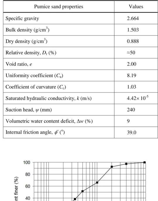
representative sample is presented in Fig. 3.3. Based on the Unified Soil Classification System, this sample is classified as a well graded sand, which has a uniformity coefficient (Cu) greater than 6 (Cu= 8.19), and a coefficient of curvature (Cc) between 1 and 3 (Cc=1.06).

Mechanical properties of the soils were obtained using static triaxial compression tests through a consolidated-undrained procedure. Pumice sand samples were remoulded to obtain five cm diameter and 10 cm high specimens with original in situ density. To achieve the required density, the determined amount of the dry sample was inserted into a mould of specified volume, using dry pluviation method. In cases where there was excess soil mass, the moulds were impacted slightly to provide extra space for the remaining soil mass. The specimens were then infiltrated with CO2 gas to replace the air inside it before it was

saturated with de-aired water. For undrained triaxial tests, Skempton (1954) introduced the pore water pressure parameter B to express the pore water pressure change Δu that occurs due

to a change in confining pressure Δ

σ

3. The Skempton’s B parameter can be obtained by

equation (3.5). 3 σ ∆ ∆ = u B (3.5)

24

Table 3.2 Pumice sand properties obtained from in-situ measurement and laboratory tests

Pumice sand properties Values

Specific gravity 2.664 Bulk density (g/cm3) 1.503 Dry density (g/cm3) 0.888 Relative density, Dr (%) ≈50 Void ratio, e 2.00 Uniformity coefficient (Cu) 8.19 Coefficient of curvature (Cc) 1.03

Saturated hydraulic conductivity, k (m/s) 4.42×10-5

Suction head, ψ (mm) 240

Volumetric water content deficit, Δw (%) 9

Internal friction angle, φ′ (o

) 39.0

25

Full saturation of the specimens was confirmed if Skempton’s B parameter was greater than 0.95. After full saturation was reached, the specimens were loaded axially into a triaxial cell with differing confining pressures of 20 kPa and 50 kPa, with displacement velocity of 0.7 mm/minute. The undrained strength parameters obtained are summarized in Table 3.2.

Stress-controlled cyclic triaxial tests (CTX) were performed to study the soil dynamic properties of the soils under cyclic loading. The specimen reconstitution procedures were similar to those in the static triaxial compression tests. The purpose is to study the effect of cyclic loading on the fully saturated part of the landslide mass.

The CTX were performed under undrained condition to simulate earthquake loading on pumice sand. The undrained condition can be considered if the earthquake loads apply quickly in the soil mass and there would not be enough time for any significant amount of water to flow out of the soil mass (Duncan & Wright 2005). To determine the validity of the undrained condition in CTX, Terzaghi’s theory of consolidation was used to determine the time required to achieve 99% of the equilibrium volume change by equation (3.6).

v c D t 2 99 =4 (3.6)

where t99 is the time required for 99% of the equilibrium volume change (hours), D is the

greatest distance that water must travel to flow out the soil mass (cm) and cv is the coefficient

of consolidation (cm2/hour). It is assumed that D is equal to the average height of temporary groundwater level on the sliding surface. From groundwater model, average phreatic level D

equal to 17.1 cm was obtained. The coefficient of consolidation, cv of pumice sand was

26

cm2/hour (Duncan and Wright 2005). From equation (3.6), the obtained value of t99 was

about equal to 7 hours (420 seconds).

Since the time of drainage is much longer than the earthquake duration time (≈ 60

seconds), it is reasonable to consider that there is no drainage occurs in the soil mass during seismic shaking (Towhata 2008). Therefore, in this study, this condition was adopted in undrained cyclic triaxial test to examine the undrained behavior of pumice sand under cyclic loading.

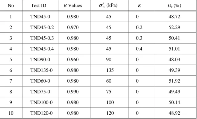
The tests were conducted at different initial effective confining pressures (σ₀′ ) and initial shear stresses, τ₀ to examine the effect of overburden pressure and ground sloping condition under cyclic loading (Table 3.3). However, to focus on field conditions, initial relative density was maintained as the in situ relative density. The ratio of initial shear stress, τ₀ to the initial effective confining pressure,σ₀′ , namely the initial stress ratio, K, is defined by equation (3.7). 0 0 σ τ ′ = K (3.7)

The test procedure was performed in a manner to simulate the stress condition in the field. At first, the specimens were consolidated with specified confining pressure after a full saturated condition has been confirmed. Initial shear stress was applied after consolidation by applying additional effective axial stress (∆ ), with open drainage and low pace loading σ₁′ (about 1kPa/minute), to ensure drained condition in the specimen. The additional axial stress given to the specimen satisfied the equation (3.8).

0

1 2τ

σ′ =

27

As an approximation of the irregular motion of earthquake loading, the amplitude of cyclic sinusoidal deviatoric axial stress, σ_d was taken to be 65% of the maximum magnitude of shear stress triggered by the actual earthquake, as proposed by Seed et al. (1975). The cyclic sinusoidal axial stresses were then applied to the specimens at a rate of 1 Hz until the ultimate failure state was achieved. Loading frequency of 1 Hz is recommended by the ASTM D5311-11 for performing dynamic test under undrained condition (Naeni and Shojaedin 2014).

Table 3.3 Summary of CTX tests conducted during this study.

No Test ID B Values σ₀′ (kPa) K Dr (%)

1 TND45-0 0.980 45 0 48.72 2 TND45-0.2 0.970 45 0.2 52.29 3 TND45-0.3 0.980 45 0.3 50.41 4 TND45-0.4 0.980 45 0.4 51.01 5 TND90-0 0.960 90 0 48.03 6 TND135-0 0.980 135 0 49.39 7 TND60-0 0.980 60 0 51.92 8 TND75-0 0.990 75 0 49.49 9 TND100-0 0.980 100 0 50.14 10 TND120-0 0.980 120 0 48.92

28

3.4 Excess pore pressure model

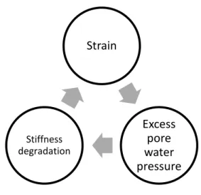
A new approach to predict excess pore water pressure by assuming reciprocal relationships between strain, stiffness and excess pore water pressure (Fig. 3.4) was developed. This approach is used for analyzing slope stability, particularly for the Tandikat pumice sands. The formulations here are based on experimental data from stress-controlled cyclic triaxial tests, using the samples from the study area. The effects of initial shear stress were also included in the analysis, to develop a reliable constitutive model for sloping ground conditions.

The role of shear strain on liquefaction and stiffness degradation has been confirmed in many researches. Lenart (2008), Jafarian et al. (2012) and Green et al. (2000) assessed strain energy-based excess pore water pressure generation by considering strain-stress relationship. Lee and Sheu (2007) proposed stiffness degradation model, which depends on cyclic strain history under cyclic straining. In this study, shear strain is assumed to be the leading factor of pore pressure increase, which consequently reduces shear stiffness as effective confining pressure decreases. However, the subsequent degraded stiffness value generates larger strain at the next loading cycle, which increases pore water pressure more rapidly (Fig. 3.4). In detail, since saturated soil at the sliding surface surpasses its elastic threshold during early cyclic loading, the soil structure contracts, and pore water pressure increases. The cyclic loading causes irreversible grain arrangement, and generates permanent excess pore water pressure. The increase of pore water pressure reduces effective stress, which consequently degrades the shear stiffness of the soil structure. At the next cycle, the soil structure is then subjected to the next loading, with current degraded shear stiffness leading to larger strain, which thus increases the pore water pressure. This behaviour is considered to be a reciprocal relationship between plastic strains, excess pore water pressure increase and shear stiffness

29

degradation, which continues on every loading cycle. Based on this principle, cycle by cycle calculation procedure considering shear stiffness and strain dependency was performed. The predicted excess pore water pressure was then used in slope stability analysis, using actual earthquake acceleration.

Fig. 3.4 Calculation scheme of strain, excess pore pressure and stiffness degradation

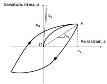
Fig. 3.5 represents an idealized stress-strain loop for a specimen subjected to symmetric cyclic loading at the first cycle. This stress-strain loop is typically obtained from a routine CTX test, where the loop is related to the maximum values of cyclic axial strain and cyclic deviatoric stress. Curve OA is defined as the initial backbone curve, which characterizes stress-strain behaviour. The backbone curve has its initial slope (E0) at the origin; this slope is

known as the maximum Young’s modulus. The secant Young’s modulus (Es) is represented

as the slope of the line connecting the original point with the tip of the loop associated with the axial strain amplitude (εs). The secant Young’s modulus (Es) and axial strain amplitude

(εs) are the key properties of the developed non-linear constitutive model. These parameters

were obtained at every cycle loading, to be correlated with the pore water pressure increase. Strain Excess pore water pressure Stiffness degradation

30

To better incorporate the earthquake motion and the developed model, the term of shear stress and shear modulus was used instead of deviatoric stress and axial strain, although the data were obtained through triaxial tests. Assuming the soil behaves isotropically and elastically, the values of the secant shear modulus, Gs, and the shear strain amplitude, γs, are

defined by the equations (3.9) and (3.10):

) 1 ( 2 s υ + = E G_s (3.9) ) 1 ( s s ε υ γ = + (3.10)

where υ is the Poisson’s ratio equal to 0.5 for undrained conditions, and Es, Gs, εs and γs are

the secant Young’s modulus, the secant shear modulus, axial strain amplitude and the shear strain amplitude, respectively. The initial shear modulus, G0, can be referred to equation (3.9)

by changing parameter Es to E0.

31

3.5 Stochastic slope stability and landslide volume analysis

3.5.1 Introduction

In the stochastic analysis, the parameters used are defined as random variables. Random variables represent the uncertainty in the nature. Synthetically, these random variables were generated by Monte-Carlo simulation through software computation that is able to produce random numbers. The generated random variables can satisfy the given probability density function (i.e., normal distribution, log-normal distribution, etc.) by previously determining the mean and standard deviation of the parameters taken from field and laboratory test. Subsequently, the random variables were used in both groundwater model and slope stability evaluation to produce probability of particular landslide hazard.

3.5.2 Groundwater modelling

Many researches have been conducted to develop numerical model to predict groundwater in unconfined aquifer. Among many methods, Boussinesq equation is most often used to estimate groundwater (Bansal and Das 2010). The performance of this method is reliable to predict experimental soil flume test (Steenhuis et al 1999; Sloan and Moore 1984). This method is generally formulated as a parabolic nonlinear partial differential equation. Thus, finite difference numerical model can be used to utilize the aforesaid equation (Bansal 2014).

The Boussinesq formula as the governing equation of the model is written as equation (3.11) (Bansal 2014).

32 t h S R x h x h h x k ∂ ∂ = +       ∂ ∂ −       ∂ ∂ ∂ ∂ _θ 2_θ cos tan ) 11 . 3 (

where h is the height of phreatic surface measured above the impermeable sloping bed in the vertical direction. k and S respectively are the hydraulic conductivity and specific yield of the aquifer. R is the net rate of recharge of infiltrated rainfall, and θ is the slope angle.

Fig. 3.6 Scheme of groundwater model by rainfall infiltration

The nonlinear Boussinesq equation can be solved numerically using the Mac Cormack scheme of explicit finite difference method (Bansal 2014). This can be done by modifying the equation (3.11) to equation (3.12): S R x h C x h h x C t h + ∂ ∂ −       ∂ ∂ ∂ ∂ = ∂ ∂ 2 1 ) 12 . 3 (

33

where,C₁ =(kcos2θ)/S and C₂ =(ksin2

θ

)/2S. Mac Cormack scheme is an explicit finite difference with predictor-corrector step. The predictor step is applied by replacing the spatial and temporal derivatives by forwards difference to obtain predicted value of h, indicated as

• h in equation (3.13).

[

]

(

)

t S R h h x t C h h h h h h x t C h hnt nt n t n t nt nt nt n t n t − nt + ∆ ∆ ∆ − − − − ∆ ∆ + = _{+ + − +} • +1 , 1 2 1, 1, , , , 1, 2 1, , , ( ) ( ) ) ( ) 13 . 3 (

where, subscript n and t are respectively spatial and time identifier. The corrector step is then obtained by replacing the space derivative by rearward difference, while the time derivative is preserved using forward difference approximation. Then equation (3.14) can be obtained.

[

]

(

)

t S R h h x t C h h h h h h x t C h h_{nt nt nt n t nt n t nt n t nt} − _{n t} + ∆ ∆ ∆ − − − − ∆ ∆ + = • + − • + • + − • + • + − • + • + + • + • • +1 , 1 2 , 1 1, 1 , 1 1, 1 , 1 1, 1 2 , 1 1, 1 , ( ) ( ) ) ( (3.14)

The final value of h_n,t+1 is simply obtained from arithmetic mean of h_n•_,t+1and h_n•_,t•₊₁from equations (3.13) and (3.14), respectively, and the equation (3.15) is obtained.

(

)

  ₋ ∆ ∆ − + = • + − • + • + +1 , , 1 2 , 1 1, 1 , 2 1 t n t n t n t n t n h h x t C h h h

(

)

(

)

{

}

t S R h h h h h h x t C _{nt n t nt n t nt n t }+ ∆   − − − × ∆ ∆ + • + − • + • + − • + • + + • +1 1, 1 , 1 1, 1 , 1 1, 1 , 2 1 ) ( (3.15)

The applied initial condition was used such as to simulate the water table condition in dry condition. Thus, the initial and boundary condition are defined by equations (3.16), (3.17) and (3.18).

34    − > − < − + = = 0 0 0 ( )tan , , 0 ) 0 , ( x L x x L x L x z t x h θ ) 16 . 3 ( 0 ) , 0 ( t = h (3.17) 0 ) , (L t z h = (3.18)

To accommodate the stochastic analysis, hydraulic conductivity parameter, k, was defined as random variable. The data of hydraulic conductivity were taken from field test. They are the base to determine statistical parameter for random variable generation.

The specific yield S, was defined as indirect random variable since it was assumed as dependent variable of hydraulic conductivity. The relationship between parameter k and S was established by Kozeny-Carman in equation (3.19) (Odong 2007).

2 10 2 3 3 ) 1 ( 10 3 . 8 d n n g k _      − × × = − η ) 19 . 3 (

where g is the gravitational acceleration (=9.807 m/s2), η is the kinematic viscosity of water at 20o C (10-6 m2/s), n is the effective porosity, and D10 is the effective grain size in mm,

relative to which 10% is finer. The specific yield, S, was then estimated from relation curve provided by Eckis (1934) in Robson (1993). By taking the coarse sand as the category of the soil, then equation (3.20) is used.

03 . 0 − ≈ n S _(3.20)

The abovementioned equation is used to define the relation between effective porosity and specific yield in groundwater model. In the stochastic analysis, specific yield is

35

dependent parameter to hydraulic conductivity which was set as random variable. Therefore, specific yield parameters are automatically counted as random variables.

Figure 3.7 shows the combined results of infiltration analysis and groundwater model. The rainfall was considered as the input in groundwater model after the depth of wet front surpasses the average thickness of pumice deposit (2.5 m). From Fig. 3.7, the base of pumice layer remained saturated after the rainfall stopped up to 16 hours. This is considered as the critical period in which the slope stability could dramatically decreases when earthquake comes.

36 3.5.3 Slope stability analysis

Slope stability analysis can be achieved by wide range alternatives from simple single-free-body (i.e. infinite slope assumption) to more complicated procedures of slices. The aforesaid procedures include such methods as the Janbu’s Simplified method, the Simplified Bishop procedure, and Spencer’s procedure (Duncan and Wright 2005). All procedures of slice techniques basically are very similar. The differences between the methods are the considered equation of statics use in the calculation, and the assumption for the interslice forces (Krahn 2004).

In the standpoint of shallow landslide, many researches use infinite slope procedure to simplify slope stability calculation. These researches use some assumptions that may appropriately support the effectiveness of infinite slope procedure, for example: slope failure by homogeneous rainfall infiltration (Iverson 2000; Agus and Liao 2009) and infinite slope with steady seepage parallel to the slope (Romeo 2000). Because the problem deals with varying seepage along the slope, the analysis cannot be appropriately analyzed with infinite slope assumption, thus more rigorous procedure was considered. This paper designated Janbu’s Simplified method which can satisfy horizontal force equilibrium, but ignores interslice shear force. The selection of Janbu’s Simplified method is based on the following reasons: 1) procedures of slice can be easily dealt with finite difference groundwater model that as well include spatial partition in the analysis; 2) shallow landslides mostly consist of planar type of slip surface. At this kind of slip surface, force equilibrium is completely independent of interslice shear force (Krahn 2004); 3) Rapid calculation is necessary to deal with the probabilistic Monte-Carlo simulation. The simulation needs numerous trials to obtain a reasonable result, thus the simplicity of the Janbu’s Simplified method ensuring the

37

shorter time of calculation. The factor of safety in the stochastic analysis is defined as FSJ, to

be attributed to Janbu’s Simplified method.

In this study, the objective to utilize the slope stability analysis is somewhat different from the common purpose. Instead of evaluating the factor of safety, the slope stability analysis is used to calculate the potential amount of sliding mass due to earthquake acceleration in particular groundwater condition. The amount of sliding mass is termed as

specific volume ratio (Rsv) that defined the displaced volume divided by the maximum

volume per unit width that could collapse from the slope (Fig. 3.8). The specific volume ratio, Rsv can be formulated by equation (3.21).

max S V

V

R_sv = (3.21) where VS is the specific volume of displaced mass when the factor of safety (FSJ) is smaller

than one, and Vmax is the probable maximum specific volume that could collapse from the

38

Fig. 3.8 Scheme of slope stability analysis

The factor of safety of Janbu’s Simplified method is obtained from equation (3.22) (Krahn 2004):

(

)

∑

∑

∑

+ − + = W k N ub N b c F h SJ sin cos ' tan ) ( cos ' θ θ φ θ (3.22)

where c′ is effective cohesion, φ'is effective angle of friction, u is pore-water pressure, kh is

the horizontal seismic coefficient applied through the centroid of each slide, W is the slice weight and N is slice base normal force, which is defined by equation (3.23).

SJ SJ ' tan sin cos ' tan sin sin ' F F ub b c W N _{θ φ} θ φ θ θ + + − = (3.23)

The base normal force, N needs to be determined using iteration process since the factor of safety (FSJ) is unknown at the first step of calculation.

39

The input of pore water pressure (u) to calculate factor of safety is taken from previously discussed groundwater model. The pore water pressure can be simply formulated as equation (3.24).

θ γ 2

whcos

u = (3.24)

where h is the groundwater height taken from groundwater simulation and γw is unit weight

of water.

3.5.4 Monte-Carlo Simulation

In Monte-Carlo simulation, a large number of replicate analyses are made using random variables that are generated in such a fashion as to approximate their defined distributions to simulate the process of sampling. An advantage of Monte-Carlo simulation is that distributional shapes (such as lognormal) can be modeled explicitly by generating random values in a manner that approximates the distribution.

Trials were repeated many times in the Monte-Carlo simulation. Once large number of runs have been completed, it is possible to study the specific volume ratio, RSV statistically.

In this study, the number of trials is 1,000 times after considering time consumption for computation.

Monte-Carlo simulation was applied to generate random variable into both groundwater model and slope stability analysis. The Monte-Carlo simulation was applied as subroutine in the main program of groundwater model and slope stability analysis to generate random parameters (Fig.3.9). All the calculations were performed by Visual Basic of Application code of Microsoft Excel (© Microsoft Corporation) which is a powerful and convenient tool

40

for both programming and data analyzing. However, to enable gradual checking of the groundwater simulation result, the calculations were performed separately (Fig.3.9).

41

Chapter 4

Initiation mechanism of the Tandikat landslide

To study about the initiation mechanism of the Tandikat landslide, several tests and analyses were conducted. This chapter discuss the results of static triaxial tests and cyclic triaxial tests (CTX), and the implementation of tests result to numerical analyses. The static triaxial tests were proposed to obtain strength parameter of pumice sand to be used in stability analysis, while the CTX were conducted to build empirical pore water pressure model to be implemented in the numerical analysis.

4.1 Result of static triaxial test

Static triaxial tests were conducted to attain the shear strength of the pumice sand, and to understand its basic physical behaviour under stresses. Initial confining pressure of 20 kPa and 50 kPa were used to nearly replicate the shallow pumice sand layer. The stress path (Fig. 4.1) shows a large sector of contractive curve, implying the effect of pore water pressure increase. It also indicates a low elastic threshold (ET), suggesting that the soil structure contracts easily under low shear stress. As the effective confining pressure decreases, the stress path exhibits dilation behaviour as it approaches the phase transformation line (PTL). Dilation behaviour implies that the soil particle undergoes densification process, which temporarily gains its stiffness. This tendency of dilation after passing PTL suggests cyclic mobility behaviour when cyclic loading is applied (Ishihara 1985). From the test, the internal friction angle (φ') is equal to 39.0°.

42

Fig. 4.1 Effective stress paths and transformed strength envelope obtained from the static triaxial tests

4.2 Typical result of cyclic triaxial test

Consider a saturated soil specimen which is consolidated under a confining pressure of

σ

3 as depicted in Fig. 4.2. The stresses in a soil specimen are change during the test such that

the axial stress is equal to σ σ_d

2 1

3 + and the radial stress is σ3 −1₂σd (Das and Ramana,

2011). The stresses on the plane X-X are σ₃ and σ_d

2 1

+ , as total normal stress and shear

stress, respectively. This state of stresses is the appropriate condition to simulate horizontal earthquake movement where shear stress working on a plane with constant total normal stress.

43

Fig. 4.2 Scheme of cyclic shear stress on a plane for a triaxial test specimen (modified from Das and Ramana, 2011)

However, in practice, it is difficult to obtain excess pore water pressure occurring in the shear plane since the placement of pore pressure sensor is at the bottom of specimen. Therefore, corrected pore pressure ratio ru is used by eliminating the effect of deviatoric

stresses at the bottom of the specimen. Corrected excess pore water pressure ratio was obtained by equation (4.1) (Zlender and Lenart 2005).

            ′ − ∆ = 0 d u 2 σ σ u B r (4.1)

where B is Skempton’s pore water pressure parameter, Δu is the excess pore water pressure,

d

σ is the deviatoric axial stress, and σ₀′ is the initial effective confining pressure.

The development of axial strain, the deviatoric stress-strain loop and the excess pore water pressure ratio during a CTX test of pumice sand under 45 kPa initial effective

44

confining pressure are shown in Figs. 4.3, 4.4 and 4.5, respectively. The shear-strain loop shows that the greatest stiffness occurred in the first stage of loading, and gradually decreased as cyclic loading proceeded. The stress path confirms cyclic mobility behaviour, where the excess pore pressure ratio rapidly increase in the first cycles, but did not necessarily reach liquefaction state until a large number of cycles had been completed (Fig. 4.6). Cyclic mobility occurred due to dilation at low level mean effective confining pressure, where the pore water pressure decreased and the mean effective confining pressure temporarily regained as the stress path passed the PTL. However, the specimen has already undergone larger strain before liquefaction was attained.

Fig. 4.3 Time history of cyclic axial strain at σ₀′ = 45 kPa

45

Fig. 4.5 Time histories of excess pore water pressure ratio at σ₀′ = 45 kPa

Fig. 4.6 Effective stress path (ESP) of mean effective confining pressure and shear stress at

0

σ′ = 45 kPa

Fig. 4.5 shows the rapid increase of pore water pressure ratio at early cycles when the axial strain (Fig. 4.3) gradually increase simultaneously. It shows that the excess pore water pressure ratio increase is influenced by amplitude of axial strain, irrespective with the direction of the loading. Therefore, in this study, the term of cumulative strain was used to evaluate the pore water pressure increase. Shear strain was used to better incorporate the

46

earthquake motion and the developed model instead using the axial strain. Cumulative shear strain was defined in equation (4.3) as the integration of shear strain amplitude by time.

∫

= = = n t t t dt 0 s t γ γ (4.2)

where γs are the shear strain amplitude and tn is the time of nth step.

To assess shear strain and excess pore water pressure increase in relation to initial effective confining pressure and initial shear stress, a reference cumulative shear strain was designated as the cumulative shear strain where ru = 0.80, which is the inflation point of the

γt-ru curve. Cumulative shear strain corresponding to ru = 0.80 was considered to be the

reference cumulative shear strain, γr, where, beyond this point, the pumice sand specimen

underwent large strain without further significant excess pore water pressure increase (Fig. 4.7).

47

4.3 Effect of initial effective confining pressure on reference cumulative

shear strain

As described in Table 3.3, the pumice sand samples were isotropically consolidated to seven different initial effective confining pressures, with σ₀′ equal to 45 kPa, 60 kPa, 75 kPa, 90 kPa, 100 kPa, 120 kPa and 135 kPa. As shown in the γt-ru plots, at each given initial

effective confining pressure, excess pore water pressure ratio increased rapidly at low cumulative shear strain (Fig. 4.8). However, each initial effective confining pressure responded differently to excess pore water pressure ratio increase during cyclic loading. Excess pore water pressure ratio of the specimen with low confining pressure increased rapidly in response to cyclic loading, whereas excess pore water pressure ratio at high confining pressure had a slower response to cyclic loading. At a given cumulative shear strain, excess pore water pressure ratio clearly increases with decreasing initial effective confining pressure (Fig. 4.8).

Figure 4.9 shows the correlation of σ₀′ and γr where γr increased with initial effective

confining pressure, indicating that more cumulative strain was necessary to increase excess pore water pressure at some level, as σ₀′ _{increased. This suggests, therefore, that shallow} saturated pumice sand deposits have higher risk of excess pore water pressure increase during earthquakes than deeper saturated sands.

48

Fig. 4.8 Excess pore water pressure versus cumulative shear strain for various initial effective confining pressures