- 65 - IEEE Workshop on Nonlinear Circuit NetworksDecember 13-14, 2013

Investigation of Behavior of Death of Neuron and Neurogenesis in Multi-Layer Perceptron

Yuta Yokoyama, Chihiro Ikuta, Yoko Uwate and Yoshifumi Nishio Department of Electrical and Electronic Engineering, Tokushima University

2-1 Minami-Josanjima, Tokushima-shi, Tokushima, 770-8506, Japan Email: { yuta, ikuta, uwate, nishio } @ee.tokushima-u.ac.jp

Abstract— It is said that there are about 100 billion neurons in

the human’s brain. However, neurons had been considered to be lost with age until several years ago. Death of neurons are can be occurred by various things. And, the neurogenesis improves ability to solve problems. In the previous study, we have proposed artificial neural network which was applied the neurogenesis.

In this study, we investigate the influences of the death of neuron and neurogenesis in more detail. We propose the death of neuron and neurogenesis during the MLP learning process.

Then, we focus on the connection weights of the neuron from the input layer to the hidden layer. We choose the neuron between the input and hidden layer. After that, the neuron is deleted from the network and the new neuron is generated. We compare the learning performance of each MLP by some MLPs.

I. I

The network of the human’s brain is formed by connecting of more than one neuron. It is said that there are about 100 billion neurons in the human’s brain. However, neurons had been considered to be lost with age until several years ago.

Namely, some neurons are generated in the brain at the infant stage. In recent studies, some researchers reported that new neurons are generated in the dentate gyrus of hippocumpus [1] - [3]. This process is called “neurogenesis”. By utilizing the neurogenesis, some brain cells increase and the network of within is substantial. It is known that the neurogenesis improves ability to solve problems by combining new neurons.

We focus on the characteristic of the neurogenesis. In the previous study, we have proposed artificial neural network which was applied the neurogenesis [4] - [6]. Therefore, we have researched the performance of the proposed network.

In this study, we focus on the characteristics of the death of neuron and neurogenesis. We apply the behavior of the death of neuron and neurogenesis to the MLP learning process. We choose the neuron which is the smallest action between the input and hidden layer. Then, the neuron is deleted from the network and the new neuron is generated at there. And, the new neuron is generated in the bottom of the hidden layer.

Therefore, we investigate the influences of the death of neuron and neurogenesis in more detail.

II. N

N

A. Death of neuron and Neurogenesis

Before, neurons had been considered to be lost with age.

Some neurons die in the adult human’s brain. Death of neurons are can be occurred by various things. However, there is no

neural stem cell which makes a neuron in the brain of an adult. It was impossible to generate the new neuron. Therefore, the neurogenesis had been considered to generate for period of growth. However, some researchers reported that new neurons are generated in the adult brain. This process is called

“neurogenesis”. The neurogenesis in the hippocumpus of the human brain was discovered in the late 1990s by Erickson et al [1] - [3]. The neurogenesis is included in the existing neural circuit by given the learning and new neurons are generated in the human brain. It is known that the neurogenesis improves memory, learning, thinking ability, and so on. We focus on the behavior of the death of neuron and neurogenesis to the learning performance during the learning.

B. Neurons Updating

We use a Multi-Layer Perceptron (MLP) which is compar- atively easy network for artificial neural network and one of a feed-forward neural network. This network is used for pattern recognition, time series prediction, noise reduction, motion control, and other tasks. The MLP is composed some layers of neuron, it has input layer, hidden layer, and output layer. This network learns to the tasks by changing the weight parameters.

Generally, the performance of the MLP is changed by the number of neurons. Moreover, we used the Back Propagation (BP) which is one of the MLP’s learning method.

A Back Propagation (BP) is used to the MLP’s learning algorithm. The BP was introduced by D.E. Rumelhart in 1986 [7] - [9]. In this algorithm, the network calculate the error from the output and teaching signal.

The neuron has the multi inputs and a single output. In this study, we use the method of MLP and BP. The updating rule of neuron is described by Eq. (1).

x

(t + 1) = f



 ∑

j

w

(t)x

(t) − θ



 , (1)

where x is the input or output and w is the connection weight parameter and θ is threshold. In this equation, the weight of connection and threshold of neuron are learned by BP algorithm. We used the sigmoid function for the output function. The error of MLP propagates backward in the feed-forward neural network. BP algorithm changes value of weights to obtain smaller error than before. The total error

- 65 -

IEEE Workshop on Nonlinear Circuit Networks December 13-14, 2013

E of the network is described by Eq. (2).

E = 1 2

∑

∑

(t

− o

)

, (2) where E is the error value, p is the number of the input data, n is the number of the neurons in the output layer, t

is the value of the desired target data for the pth input data, and o

is the value of the output data for the pth input data. The function of the connection weight is described by Eq. (3).

∆

w

= η

o

= − η ∂E

∂w

, (3) where w

is the weight between the ith neuron of the layer k − 1 and the j the neuron of the layer k, and η is the proportionality factor known as the learning rate.

C. Proposed Network

In this study, we investigate in more detail the influences of neurogenesis. We apply the behavior of the death of neuron and neurogenesis to MLP. We use that the MLP is composed of three layers (one input, hidden, and output layer). We propose the death of neuron and neurogenesis during the MLP learning process. Then, we consider characteristics of the extinction, death of neuron and generated neurons.

(a) Conventional network. (b) Death of neuron and replaced neurogenesis.

(c) Death of neuron and additional neurogenesis.

Fig. 1. Network models.

We explain how to generated neurogenesis and death of neurons. We focus on the connection weights of the neuron from the input layer to the hidden layer. Then, we consider two kind of the death of neuron and neurogenesis. One is the death of neuron and replaced neurogenesis. In this network, we choose the neuron which is the smallest action between the input and hidden layer. After that, the neuron of the smallest action is deleted to the network and the new neuron is generated at there. This process is called “death of

neuron and replaced neurogenesis”. The other is the death of neuron and additional neurogenesis. This network is carried out in the similar method of the death of neuron and replaced neurogenesis. However, new neuron is generated in the bottom of the hidden layer after the neuron of the smallest action is deleted and generated during the learning process. Namely, this net work is additional neurogenesis while the neuron is deleted and generated. Then, all connection weights to the generated neurons are newly set small random values.

In this study, we assume the process to generated neurons and connection to “neurogenesis”. After that, the connection weights are newly calculated. Figure 1 (b), (c) show a structure of the proposed network.

III. S

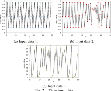
In this study, we apply the learning of the time series to MLP learning process. We use the chaotic time series produced by the logistic map. We compare the learning performance of the each MLPs. Figure 2 shows the three input data.

(a) Input data 1. (b) Input data 2.

(c) Input data 3.

Fig. 2. Three input data.

We set that the conventional network and the proposed network are composed of three layers. The number of neurons in the input layer and the output layer are 50 neurons. Then, we set that the conventional MLP has 5 neurons in the hidden layer. In the MLP with death of neuron and additional neuroge- nesis, we set to 5 neurons in the hidden layer at the start of the learning process. Therefore, the proposed MLP is set that the number of neurons in the hidden layer increases. And, we set the maximum number of the neurons in the hidden layer. The MLPs learn 10000 times during the one trial. The learning rate of the existing neuron is η = 0.005 and the generating neuron is 0.05. We set the timing that we choose the smallest action of neuron at every 750 iterations. The initial value of the weights of existing neuron are given between -1.0 and 1.0 Similarly, the generating neuron are given between -0.5 and 0.5 at random. Because, we consider that the neurogenesis is possible to many learning. We compare the learning performance of the following three kinds of MLPs:

- 66 -

1) The conventional MLP

2) The MLP with death of neuron and replaced neurogen- esis (MLP - DR)

3) The MLP with death of neuron and additional neuroge- nesis (MLP - DRA)

We use a Mean Square Error (MSE) as the measure of their performances. MSE is defined by Eq. (4).

M SE = 1 N

∑

(t

− o

)

. (4) We make a comparison between the three MLPs. We investigate the learning in some approaches.

A. Example of the learning performance

In this section, we compare the example of the learning performance of the three different MLPs. We show an example of the learning performance of the MLPs in Figs. 3 and 4.

In this example, we set the neurons in the hidden layer that the conventional MLP and the MLP - DR is set to 5 and 15 neurons. Therefore, the MLP - DRA is set the neuron in the hidden layer that the number of neurons increases until 15 neurons during the learning process. We show these results of the learning performance when we set that same initial value of the weight connections.

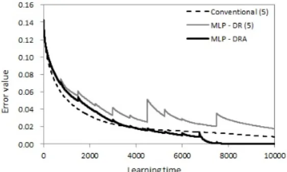
Fig. 3. Example of learning performance (5 neurons in the hidden layer).

Fig. 4. Example of learning performance (15 neurons in the hidden layer).

In Fig. 3, we show the example of the learning performance when we set the conventional MLP and the MLP - DR with 5 neurons in the hidden layer. In the MLP - DRA, we set to 5 neurons in the hidden layer at the start of learning. During the learning process, neurons in the hidden layer are deleted and generated until 15 neurons. Similarly, we show the example of the learning performance when we set the the conventional

MLP and the MLP - DR with 15 neurons in the hidden layer in Fig. 4.

From Figs. 3 and 4, the error of each MLP decreases. Then, we focus on the value of the error at the last of learning time.

The learning performance of the MLP - DRA is better than the conventional MLP. We considered that the behavior of the death of neuron and neurogenesis can be applied well.

However, we can say that the learning performance of the MLP - DR obtains negative result in Fig. 3. Therefore, we consider that the death of neuron and neurogenesis have adverse effects on the small number of neurons in the hidden layer.

B. Average of the learning performance

In this section, we compare the average of the learning performance of the three different MLPs. Moreover, we carry out 100 trials with different initial weights of connections. We used the conventional MLP and the MLP - DR with 5 and 15 neurons in the hidden layer. In the MLP - DRA, we set to 5 neurons at the start of the learning process. We show the average of the learning performance of the MLPs in Table I.

TABLE I

AVERAGE OF THE LEARNING PERFORMANCE (1) The conventional MLP.

Neurons Average Minimum Maximum Standard variation

5 0.00841 0.00301 0.01793 0.00374

15 0.00135 0.00075 0.00322 0.00044

(2) The MLP - DR.

Neurons Average Minimum Maximum Standard variation

5 0.00935 0.00020 0.02896 0.00764

15 0.00101 0.00004 0.00754 0.00136

(3) The MLP - DRA.

Neurons Average Minimum Maximum Standard variation 5→15 0.00094 0.00005 0.00522 0.00126

In Table I (1), we show the average of the learning perfor- mance of the conventional MLP. We consider that the learning performance of the 15 neurons in the hidden layer is better than 5 neurons in the hidden layer. And, we show the average of the learning performance of the MLP - DR in Table I (2).

Then, we compare the conventional MLP and the MLP -DR with 5 neurons in the hidden layer. In this comparison, we can see that the average of the learning performance of the MLP - DR obtains negative result from Table I (1), (2). Similarly, we compare the conventional MLP and the MLP - DR with 15 neurons in the hidden layer. In this comparison, we can see that the average of the learning performance of the MLP - DR is better than the conventional MLP from Table I (1), (2).

Namely, we can show the minimum error of the MLP - DR is smaller than the the conventional MLP. From these results, we consider that the death of neuron and replaced neurogenesis have adverse effects on the small number of neurons in the hidden layer.

In Table I (3), we show the average of the learning perfor- mance of the MLP - DRA. We compare the conventional MLP

- 67 -

with 15 neurons, the MLP - DR with 15 neurons in the hidden layer and the MLP - DRA. In this comparison, we can show that the learning performance of the MLP - DRA is the best result of all MLPs. Moreover, we can see that the minimum error of the MLP - DRA is the smallest value. Because, we consider that the parameter of the connecting weight changed by the behavior of the death of neuron and neurogenesis. Thus, we consider that the death of neuron and neurogenesis have a positive effect on the this network and the learning process.

C. Output data of the learning process

In this section, we compare the output data of the learning process of the conventional MLP with 15 neurons in the hidden layer and the MLP - DRA. We give the same initial value in the each MLP. We compare the target data when we set the second pattern of the input data 2. Then, we show the error value and the processing time in Table II at these results. At the same moment, we show the example of the target data and output data of the each MLP in Figs. 5 and 6 when we obtain the error value in Table II.

TABLE II LEARNING PERFORMANCE

(1) The conventional MLP. (2) The MLP - DRA.

Network model Neurons Error value Processing time

(1) 15 0.00167 0.86

(2) 5→15 0.00072 0.76

Fig. 5. Comparison of the target data and the output data of the conventional MLP (Target data 2).

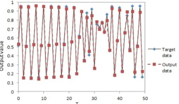
Fig. 6. Comparison of the target data and the output data of the MLP - DRA (Target data 2).

In Fig. 5, we show the example of the target data and output data when we set that the conventional MLP with 15 neurons in the hidden layer. Similarly, we show the example of the

target data and output data when we set that the MLP - DRA in Fig. 6.

From Figs. 5 and 6, we compare the output data of the each MLP. We can say that the each MLP has approximated the target data. However, we can show that the MLP - DRA is more approximate than the conventional MLP to the target data. Namely, we are able to obtain the good performance by the proposed network. Because, we consider that the error value of the MLP - DRA is smaller than the conventional MLP from Table II. At the same moment, we are able to obtain that the processing time of the MLP - DRA is a few faster than the conventional MLP. Because we used the small number of neurons in the hidden layer at the start of learning process.

IV. C

In this study, we proposed the MLP - DR and MLP - DRA for the death of neuron and neurogenesis during the MLP learning process. In the proposed network, we chosen the neuron between the input and hidden layer. After that, the neuron was deleted from the network and the new neuron is generated. We compared the learning performance of each MLP by some MLPs.

In some simulations, we were able to obtain the good performance of the proposed network. We can see that the death of neuron and neurogenesis have a positive effect on the this network and the learning. Because, we considered that the parameter of the connection weight changed by the behavior of the death of neuron and neurogenesis. Therefore, we can say that the death of neuron and neurogenesis have a positive effect on the this network and learning process.

R

[1] S. Becker, J. M. Wojtowicz, “A Model of Hippocampal Neurogenesis in Memory and Mood Disorders,” Cognitive Sciences, vol. 11, no. 2, pp. 70-76, 2007.

[2] R. A. Chambers, M. N. Potenza, R. E. Hoffman, W. Miranker, “Simu- lated Apotosis/Neurogenesis Regulates Learning and Memory Capabili- ties of Adaptive Neural Networks,” Neuropsychopharmacology, pp. 747- 758, 2004.

[3] H. Satoi, H. Tomimoto, R. Ohtani, T. Kondo, M. Watanabe, N. Oka, I. Akiguchi, S. Furuta, Y. Hirabayashi and T. Okazaki, “Astroglial Expression of Ceramide in Alzheimer’s Disease Brains: A Role During Neuronal Apoptosis,” Neuroscience, vol. 130, pp. 657-666, 2005.

[4] Y. Yokoyama, T. Shima, C. Ikuta, Y. Uwate and Y. Nishio, “Improvement of Learning Performance of Neural Network Using Neurogenesis,”

Proceedings of RISP International Workshop on Nonlinear Circuits and Signal Processing (NCSP’12), pp. 365-368, Mar. 2012.

[5] Y. Yokoyama, C. Ikuta, Y. Uwate and Y. Nishio, “Performance of Multi- Layer Perceptron with Neurogenesis,” Proceedings of International Symposium on Nonlinear Theory and its Applications (NOLTA’12), pp.715 718, Oct. 2012.

[6] Y. Yokoyama, C. Ikuta, Y. Uwate and Y. Nishio, “Investigation of Influences of Neurogenesis in Multi-Layer Perceptron,” Proceedings of International Symposium on Nonlinear Theory and its Applications (NOLTA’13), pp.382 385, Sep. 2013.

[7] D.E. Rumelhart, G.E. Hinton and R.J. Williams, “Learning Represen- tations by Back Propagation Error,” Nature, vol. 323-9, pp. 533-536, 1986.

[8] D.E. Rumelhart, G.E. Hinton and R.J. Williams, “Learning Internal Representations by Error Propagation,” Parallel Distributed Processing, vol. 1, pp. 318-362, 1986.

[9] D.E. Rumelhart, J.L. McClelland, and the PDP Research Group, “Par- allel distributed processing,” MIT Press, 1986.

- 68 -