- 72 - IEEE Workshop on Nonlinear Circuit NetworksDecember 15-16, 2017

Analysis of Frustration by Coupled Ring and Star of BVP-VDP Oscillator

Kazuki Ueta, Yoko Uwate and Yoshifumi nishio Dept. Electrical and Electronic Eng.,

Tokushima University 2-1 Minami-Josanjima, Tokushima 770-8506, Japan

Email: kazuki, uwate, [email protected]

Abstract—Synchronization phenomena of frustration network by coupled oscillators has been studied in a wide range of fields, such as BVP oscillator is the simplest mathematical model describing a neural activity. However, even if two BVP oscillators are merely completed by a linear element, the whole system exhibits complicated behavior. In this study, we focus on the synchronization phenomena coupled by Bonh¨offer-van der Pol oscillator and van der Pol oscillators (BVP and VDP) containing ring and star structures. At that time, we observe the synchronization phenomena with computer simulation.

I. I

NTRODUCTION

There are a lot of synchronization phenomena in this world.

This is one of the nonlinear phenomena that we can often observe by natural animate beings which do collective actions.

For example, firefly luminescence, cry of birds and frogs, applause of many people and so on. Synchronazation phe- nomena have a feature that the set of small power can produce very big power by synchronizing at a time. Therefore study of synchronization phenomena have been widely reported not only engineering but also the physical and biological fields[1]–

[6]. Investigation of coupled oscillators attention from many researchers because coupled oscillatory network produces in- teresting phase synchronization such as the phase propagation wave, clustering and complex patterns. In addition, it has the advantage of being able to manufacture for circuit on the board.

In this study, we focus on the synchronization phenomena coupled by Bonh¨offer-van der Pol oscillator and van del pol oscillators (BVP and VDP) containing ring and star structures.

Here, we used BVP as frustration. Then, we obserb the synchronization phenomena with computer simulation.

C C

-g

L

r C L

Fig. 1. Bonh¨offer-van der Pol oscillator and van del pol oscillator.

II. P

REVIOUS CIRCUIT MODEL

[7]

A. Circuit Model

Figure 2 shows a system model constituted van del pol oscilators (VDP-A and VDP-B) in our previous study[7]. We couple each VDP-B via inductor L and ground by coupling resistor R. In addition, we couple VDP-A via resistor r. VDP- A is the only one central circuit which is connected to all VDP-B in this system by resistor r.

VDP B

VDP A C L C

i

A

i

Ag

v

A

i

kg

v

k

VDP A

VDP B

VDP A

VDP B

VDP B

R R

R 2L

2L 2L 2L 2L

R

r r

r r

2L

Fig. 2. System model.

In the computer simulations, we assume that the voltage and current characteristics of the nonlinear resistor in each oscillator are given by the follows:

i

g

= − g

1

v + g

3

v

³

, (1) (g

₁

, g

₃

> 0).

When we coupled ring of each VDP, the feature of ring coupling has in-phase and N-phase. On the other hand, the feature of star coupling has in-phase and anti-phase.

- 72 -

IEEE Workshop on Nonlinear Circuit Networks December 15-16, 2017

First, the circuit equations of VDP-A are given as follows:

 

 

 

 C dv

A

dt = − i

A

− i

Ag

+ 1

r (N v

A

− v

1

− v

2

− ... − v

N

), L di

A

dt = v

A

,

(2)

where N denotes the number of VDP-B.

On the other hand, VDP-B is connected to the adjacent VDP- B and VDP-A. The circuit equations of VDP-B are given as follows:

 

 

 

 

 



C dv

k

dt = − i

ka

− i

kb

− i

kg

− 1

r (v

k

− v

A

), 2L di

ka

dt = v

k

− R(i

ka

+ i

k+1,b

), 2L di

kb

dt = v

k

− R(i

kb

+ i

k−1,a

),

(3)

(k = 1, 2, ..., N).

By using the following parameters and variables:

i

_A

=

√ g

₁

C

3g

3

L y

_A

, i

_ka

=

√ g

₁

C

3g

3

L y

_ka

, i

_kb

=

√ g

₁

C 3g

3

L y

_kb

, v

_A

=

√ g

₁

3g

3

x

_A

, v

_k

=

√ g

₁

3g

3

x

_k

,

t = √

LCτ, “ · ” = d

dτ , α = g

1

√ L C , β = 1

r

√ L

C , γ = R

√ C L ,

(4)

where α is the nonlinearity, β is the coupling strength between VDP-A and VDP-B. γ indicates the coupling strength between VDP-B. The normalized circuit equations of VDP-A are given as follows:

 



 

˙

x

_A

= αx

_A

( 1 − 1

3 x

²_A

)

− y

_A

+β(N x

A

− x

1

− x

2

− ... − x

N

),

˙ y

A

= x

A

.

(5)

The normalized circuit equations of VDP-B are given as follows:

 



 

˙

x

k

= αx

k

(1 − 1

3 x

²_k

) − y

ka

− y

kb

− β(x

A

− x

k

),

˙

y

_ka

= 0.5 { x

_k

− γ(y

_ka

+ y

_k+1,b

) } ,

˙

y

_kb

= 0.5 { x

_k

− γ(y

_ka

+ y

_k−1,b

) } .

(6)

B. Simulation Results

We calculate Eqs. (5) and (6) using the Runge-Kutta method with the step size h = 0.02. We show the simulation result of the synchronization phenomena when N = 4 in Fig. 3.

In this figure, we show the attractor of each oscillator and the horizontal axis is the voltage of each oscillator, and the vertical axis is the electric current of each oscillator. We set the parameters α = 0.1, β = 0.0075 and γ = 0.02. In addition, we show the system model of N = 4 in Fig. 4.

x

¹

y

¹

x

²

y

²

x

³

y

³

x

⁴

y

⁴

x

⁵

y

⁵

Fig. 3. Attractor between adjacent oscillators forN = 4 (horizontal axis:x_k, vertical axis:yk) (k = 1, 2, 3, 4, 5).

VDP B

VDP A

VDP B VDP B

VDP B

R

R

R

R 2L 2L

2L 2L

2L 2L 2L

2L r

r r

r

Fig. 4. System model ofN= 4.

Next, the time waveforms of the voltage of each capacitor C after sufficient time has elapsed are shown in Fig. 5. And the phase differences between the adjacent oscillator of this case is equal to the result as shown in Fig. 6. It seems that two electric currents of VDP-B are piled up as we underestand it from the figures like 3 phase.

x

n

time

Fig. 5. The Time waveforms of the each oscillator forN = 4.

x

1

x

2

x

1

x

3

x

1

x

4

x

1

x

5

x

2

x

3

x

2

x

4

x

2

x

5

x

3

x

4

x

3

x

5

Fig. 6. Lissajous figures ofN = 4.

Second, the simulation results of the system model con- taining six circuits are shown in Fig. 7. The value of the

- 73 -

parameters are fixed with β=0.001, 0.0085 and 0.05. In the case of β=0.001, 5 phase synchronization appeared because the coupling strength of VDP-A is weak. The current of the VDP-A and one of the current of the VDP-B are in phase at that time. Therefore, we assume 5 phase synchronization.

When the value of β sets 0.0085, some time waveforms of VDP-B come close on in-phase synchronization. When we increase coupling strength, most of two electric currents of VDP-B are piled up as we understand it from the Lissajous figures.

In the case of β=0.05, 5 phase synchronization become in- phase synchronization. And then VDP-A becomes anti-phase synchronization with VDP-B by increasing the value of β . We understand that VDP-B synchronizes even if we read either figure.

x

²

x

³

x

¹

x

¹

x

¹

x

¹

x

¹

x

⁴

x

⁵

x

⁶

(a) β=0.001.

x

²

x

³

x

1

x

1

x

¹

x

¹

x

1

x

⁴

x

⁵

x

⁶

(b) β=0.0085.

x

²

x

3

x

¹

x

¹

x

1

x

1

x

¹

x

4

x

5

x

6

(c) β=0.05.

Fig. 7.

Simulation Results for N=5 (α = 0.1 and γ = 0.02). time- waveform. Red and other colors denote x

c

and x

N

respectively. (N

= 1,2,...,6)

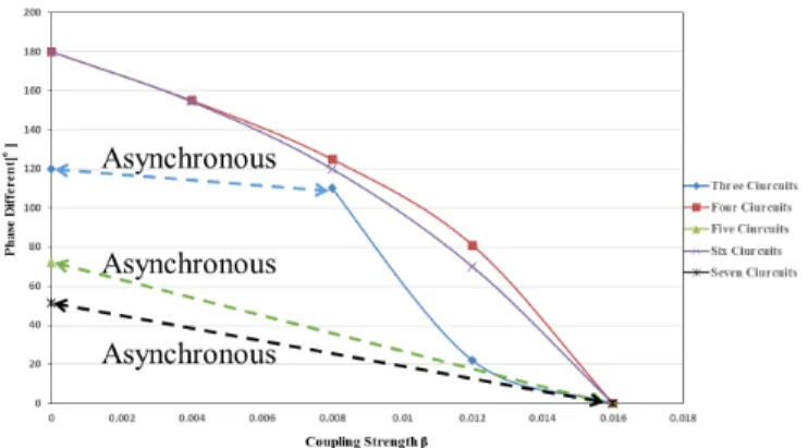
In Fig. 8, we show the results when we increase the cuircuit

numbers N = 3, 4, ..., 7. The phase difference is based on one voltage waveform of VDP-B. The broken line in the figure represent asynchronous. The solid line in the figure represent synchronous. From this result, It turns out that an even number circuits become in-phase as increasing the coupling strength.

Similarly, It turns out that an even number circuits become in-phase as increasing the coupling strength. However, we could not confirm the synchronization state between β=0 and β =0.016 in an odd number circuits.

Fig. 8.

Relationship between coupling strength and phase difference.

III. P

ROPOSED SYSTEM MODEL

Next, we propose the system model which replaces central circuit with chaotic circuit[8]. Figure 9 shows a system model constituted Bonh¨offer-van der Pol oscillator and van der Pol oscillators (BVP and VDP). A VDP is coupled adjacent VDP via inductor L and ground by coupling resistor R

0

. In addition, a VDP is coupled BVP via resistor R. BVP is the only one central circuit which is connected to all VDP in this system by resistor R.

VDP A

VDP

VDP R0

VDP VDP

BVP BVP

2L

2L 2L 2L 2L

2L

R0

R0 R

R

R R

R0

C C -g C

-g

L

r

Fig. 9. System model.

When we coupled ring of each VDP, the feature of ring coupling has in-phase and N-phase. On the other hand, the feature of star coupling has in-phase and anti-phase. Where N denotes the number of VDP. VDP is connected to the adjacent VDP and BVP.

- 74 -

Where α is the nonlinearity, β is the coupling strength of star, σ is internal parameter of BVP, γ indicates the resistive component and y

n

denotes the current of neighbor oscillator on coupling resistor R

0

. The normalized circuit equations of BVP is given as follows:

 

 



 

 

˙

x

_c

= αx

_c

( 1 − 1

3 x

²_c

)

− z

_c

− β { N x

_c

−

∑

N n=1

x

_n

} ,

˙

y

c

= z

c

− σy

c

,

˙

z

c

= x

c

− y

c

.

(7)

The normalized circuit equations of VDP are given as follows:

 



 

˙

x

_n

= αx

_n

(1 − 1

3 x

²_n

) − y

_n

− z

_n

+ β (x

_c

− x

_n

),

˙

y

_n

= 0.5 { x

_n

− γ(y

_n

+ z

_n+1

) } ,

˙

z

n

= 0.5 { x

n

− γ(y

n

+ z

n−1

) } .

(8)

IV. S

IMULATION

R

ESULT

We show the simulation result of the synchronization phe- nomena when N = 3 in Figs. 10 and 11. In Fig. 10, we show the attractor of each oscillator. The horizontal axis is the voltage of each oscillator, and the vertical axis is the electric current of each oscillator. We set the parameters α = 1.46, σ

= 1.25, γ = 0.1 and β = 0. The BVP changes from a chaotic solution to a periodic solution according to the initial value.

Therefore, Fig. 11 shows the phase difference compared in two patterns (chaotic and periodic) when we increase the coupling strength β .

x

^c

y

^c

x

1

y

1

x

2

y

2

x

³

y

³

x

^c

y

^c

x

1

y

1

x

2

y

2

x

³

y

³

Fig. 10. Attractors of chaotic and periodic solution whenβ= 0.

-180 -120 -60 0 60 120 180

0 0.02 0.04 0.06 0.08 0.1 0.12 0.14 0.16 0.18 0.2

Phase Difference of each VDP

Coupling Strength β

VDP2 Chaos MIN VDP2 Chaos MAX VDP3 Chaos MIN VDP3 Chaos MAX VDP2 Periodic MIN VDP2 Periodic MAX VDP3 Periodic MIN VDP3 Periodic MAX

Fig. 11. The phase difference among the surrounding circuits.

In Fig. 11, we show the phase difference among the sur- rounding circuits. These broken lines are chaotic solution and solid lines are periodic solution. This figure shows a com- parison between chaotic solution and periodic solution. We measured the phase difference with reference to one Poincar section. As a result, as increasing β, the chaotic solution is drawn into the periodic solution. And also, surrounding VDP synchronised in-phase according to increasing β . Since A and B are in agreement, it is considered that there is some correlation between both. Finally, as BVP is synchronized, it can be said that frustration bacame weak.

V. C

ONCLUSIONS

In this study, we have proposed the system model using Bonh¨offer-van der Pol that is combined the ring and star structures. We have observed the synchronization phenomena by increasing the coupling strength of star. When the coupling strength is sufficiently small, system model becomes like func- tion of ring coupling therefore, N phase synchronization can be observed. By increasing the coupling strength, waveforms of VDP have come close in-phase synchronization. In the future, we investigate synchronization phenomena using other circuits.

R

EFERENCES

[1] L. L. Bonilla, C. J. Paerez Vicente and R. Spigler, “Time-Periodic Phases in Populations of Nonlinearly Coupled Oscillators with Bimodal Frequency Distributions”, Nonlinear Phenomena, vol. 113, pp. 79-97, 1998.

[2] J. A. Sherratt, “Invading Wave Fonts and Their Oscilatory Wakes are Linked by a Modulated Traveling Phase Resetting Wave”, Nonlinear Phenomena, vol. 117, pp. 145-166, 1998.

[3] G. Abramson, V. M. Kenkre and A. R. Bishop, “Analytic Solutions for Nonlinear Waves in Coupled Reacting Systems”, Statistical Mechanics and its Applications, vol. 305, pp. 427-436, 2002.

[4] I. Belykh, M. Hasler, M. Lauret and H. Nijmeijer, “Synchronization and Graph Topology”, International Journal of Bifurcation and Chaos, vol.

15, no.11, pp. 3423-3433, 2005.

[5] L. M. Pecora and T. L. Carrol, “Synchronization in Chaotic Systems”, Physical Review Letters, vol. 64, pp. 821-824, 1990.

[6] L. Cveticanin, “Van der Pol oscillator with time variable parameters”, Acta Mechanica, vol. 224, pp. 945-955, 2013.

[7] K. Ueta, Y. Uwate and Y. nishio, “Frustrated Coupled Oscillators with Anomalous Coupling Method”, Proc. PrimeAsia2017, pp. 37-40, 2017.

[8] T. Ueta, H. Miyazaki, T. Kousaka, H. Kawakami, “Bifurcation and Chaos in Coupled BVP oscillators”, Bifurcation and Chaos, vol. 14, No. 4, pp.

1305-1324, 2004.

- 75 -