ShinnosukeNishi ,KenjiroTerada ,JunjiKato ,ShinjiNishiwaki andKazuhiroIzui Two-scaletopologyoptimizationforcompositeplateswithin-planeperiodicity

Published online in Wiley Online Library (wileyonlinelibrary.com). DOI: 10.1002/nme.5545

Two-scale topology optimization for composite plates with in-plane periodicity

Shinnosuke Nishi¹, Kenjiro Terada^2,*,† , Junji Kato³ , Shinji Nishiwaki⁴and Kazuhiro Izui⁴

1Department of Civil and Environmental Engineering, Tohoku University, 468-1 Aza-Aoba, Aramaki, Aoba-ku Sendai, 980-0845, Japan

2International Research Institute of Disaster Science, Tohoku University, 468-1 Aza-Aoba, Aramaki, Aoba-ku, Sendai, 980-0845, Japan

3Department of Civil and Environmental Engineering, Tohoku University, 6-6-06 Aza-Aoba, Aramaki, Aoba-ku, Sendai, 980-8597, Japan

4Department of Mechanical Engineering and Science, Kyoto University, Kyotodaigaku-katsura CIII, Nishikyo-ku, Kyoto, 615-8540, Japan

SUMMARY

This study proposes a two-scale topology optimization method for a microstructure (an in-plane unit cell) that maximizes the macroscopic mechanical performance of composite plates. The proposed method is based on the in-plane homogenization method for a composite plate model in which the macrostructure is modeled using thick plate theory and the microstructures are three-dimensional solids. Macroscopic plate charac- teristics such as homogenized plate stiffnesses and generalized thermal strains are evaluated through the application of numerical plate tests applied to an in-plane unit cell. To handle large rotations of the com- posite plates, we employ a co-rotational formulation that facilitates working with the two-scale plate model formulated within a small strain framework. Two types of objective functions are tested in the presented optimization problems: one minimizes the macroscopic end compliance to maximize the macroscopic plate stiffness, whereas the other maximizes components of a macroscopic nodal displacement vector. Analytical sensitivities are derived based on in-plane homogenization formulae so that a gradient-based method can be employed to update the topology of in-plane unit cells. Several numerical examples are presented to demon- strate the proposed method’s capability related to the design of optimal in-plane unit cells of composite plates.

Copyright © 2017 John Wiley & Sons, Ltd.

Received 6 September 2016; Revised 2 March 2017; Accepted 3 March 2017

KEY WORDS: multiscale topology optimization; analytical sensitivities; composite plates; in-plane homog- enization; co-rotational formulation

1. INTRODUCTION

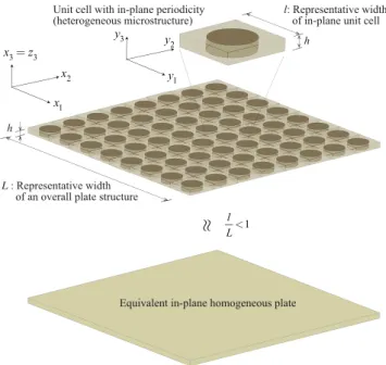
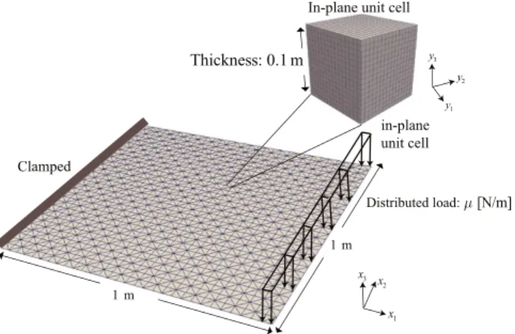
Plates with heterogeneous local structures, generally called ‘composite plates’, are actively utilized in a variety of industrial fields such as the airplane, aerospace, and automobile industries. Most com- monly, one or more types of local structures are arranged periodically in the in-plane directions, each of which can be termed an ‘in-plane unit cell’, as illustrated in Figure 1. Because the local structures determine overall structural characteristics such as bending and torsional stiffnesses, it is desirable to control their topologies is desirable, to enhance additional performances (e.g., to reduce weight and achieve a targeted flexibility). In this context, because Bendsøe and Kikuchi [1] and Suzuki and Kikuchi [2] first publicized a structural topology optimization method that incorpores a mathemati- cal homogenization theory, it has become widely utilized to determine optimal material distributions

*Correspondence to: Kenjiro Terada, International Research Institute of Disaster Science, Tohoku University, 468-1, Aramaki, Aoba-ku, Sendai 980-0845, Japan.

†Email: [email protected]

Figure 1. Concept of homogenization for composite plate with in-plane periodic microstructure.

in design regions. Comprehensive reviews of previously developed topology optimization methods can be found elsewhere; see, for example, References [3 – 6] and references therein.

In any event, most of the developments in topology optimization have addressed structures only on a single spatial scale. Although some articles are devoted to the topology optimization of microstruc- tures, only a few attempts have so far been made to study topology optimization methods that account for the interaction between macrostructures and microstructures. Nevertheless, in recent years, there has been a growing interest in such ‘multiscale topology optimization’, which depends on solving the so-called two-scale boundary value problem (BVP) derived within the framework of homogeniza- tion theory [7]. For example, Rodrigueset al.[8] propose a hierarchical approach to simultaneously determine the topologies of both macrostructures and microstructures for linearly elastic materials.

A similar approach proposed by Nakshatralaet al.[9] assumes the existence of hyperelastic materi- als in microstructures, assisted by the method of fully coupled nonlinear two-scale analyses [7]; see, for example, [10] for a more recent development. In these studies, each Gauss point or divided region of the macroscopic finite element (FE) model, whose topologies are intended to be optimized simul- taneously, is associated with a single microstructure, and the topologies of all the microstructures are determined separately.

In contrast, Huanget al.[11] present a multiscale optimization scheme for a single topology of periodic microstructures in the macrostructure, a so-called uniformly structured material, for the optimal design of cellular materials. Furthermore, Katoet al.[12] propose a multiscale topology optimization based on a decoupling multiscale analysis method for nonlinear solids [13], in which microscale and macroscale nonlinear analyses are decoupled. This method depends on the method of numerical material testing to determine a single topology within a fixed macrostructural topology.

A hierarchical approach is also taken by Vicenteet al.[14] to determine a macrostructural topology that minimizes the eigenfrequencies of the macrostructure based on the optimization of a single microstructural topology. Additional recent progress in multi-scale topology optimization methods are presented in Yanet al.[15], Xia and Breitkopf [16, 17], Longet al.[18], and Daet al.[19].

Although there has been a great deal of research has been carried out to date concerning mul- tiscale structural topology optimization, in which both microstructures and macrostructures are two-dimensional or three-dimensional (2D/3D) solids, no previous studies have presented a mul- tiscale structural topology optimization method for composite plates with in-plane unit cells. The following facts are considered to be obstacles when following this path of research:

• The standard homogenization theory for 3D solids [20, 21] assumes that 3D heterogeneous microstructures are periodic, whereas composite plates have periodicity only in the in-plane directions (Figure 1);

• Whereas the representative length of the microstructures is assumed to be infinitesimally small compared with that of the macrostructure in standard homogenization theory, the thickness of an in-plane unit cell must be the same as that of a macroscopic plate. This implies that the limit cannot be taken as the volume of the unit cell approaches zero; and

• Whereas 3D solid models are employed when formulating the governing equations at both scales in standard homogenization theory, the overall mechanical behavior of composite plates must be described using thick plate theory, in which resultant stresses must be evaluated through 3D analyses of an in-plane unit cell.

In short, multiscale modeling for composite plates with in-plane periodicity has not been fully established. In particular, the second item set forth above conflicts with the mathematical theory of homogenization [20, 21] and has never been explored. Inevitably, previous research on the optimiza- tion for composite plates has been limited to 2D optimization of in-plane periodic local structures [22] and 3D size optimization of members of sandwich panels [23, 24]. In this context, Terada et al.[25] have recently proposed an innovative two-scale analysis method for composite plates by applying the idea of numerical material testing [13] to classical thick plate theory. In their method, thick plate theory is applied to macroscopic plates, whereas a 3D solid is employed for the in-plane unit cells. The microscopic analysis for in-plane unit cells uses numerical plates testing (NPT) to

‘measure’ the homogenized thick plate stiffnesses (in-plane tension/compression/shear, bending, and torsional stiffnesses, along with transverse-shear stiffnesses). In this study, we incorporate this new and original method of NPT to construct a method for two-scale topology optimization of composite plates, to determine optimum topologies of in-plane unit cells that maximize macroscopic mechani- cal performances. In addition, the method is extended to include thermal excitation because thermal deformations are easily introduced in the current NPT format. Through the NPT method, the pro- posed two-scale topology optimization method enables us to obtain optimal topologies of in-plane periodic 3D cross-sectional structures of composite plates.

While developing the method presented here, we also wanted to consider large translations and rotation of the composite plates so that the two-scale topology optimization could be applied to design and control the functionalities of composite plates for application in actuators and other flex- ible devices. When working with such large displacements, the assumption of linear kinematics is no longer valid. In the first decade of the 2000s, certain geometrical nonlinearities were incorpo- rated into topology optimization formulations, for example, by Buhlet al.[26], Bruns and Tortorelli [27], Gea and Luo [28], Jung and Gea [29], and Cho and Jung [30]. In their reports, geometrically nonlinear problems are described using the total Lagrangian or updated Lagrangian formulations, to which finite strain is commonly introduced. However, these formulations appear to be intractable in a two-scale analysis method for composite plates [25], because the small strain framework is the premise for obtaining homogenized plate stiffnesses with NPT, and its extension to large deforma- tions is far from trivial. To manage small strains and large translation/rotation simultaneously, we employ the so-called co-rotational (CR) formulation [31 – 33], in which the motion of each plate’s FE is decomposed into two types: one for rigid body motion and the other for elastic deformation under the assumption of infinitesimal strain. In this way, in-plane homogenization [25] can be applied for the elastic deformation, and some minor adjustments are made to follow the rigid body motion.

In Section 2, we summarize the in-plane homogenization method and present formulae for com- puting the homogenized plate stiffness matrix and the macroscopic thermal stress, thus reflecting the topologies of in-plane unit cells. The CR formulation is then introduced to address large displace- ments (translations and rotations) during the in-plane homogenization process. Section 3 is devoted to the formulation of the two-scale topology optimization method. In this study, to determine one or more topologies of in-plane unit cells, we focus on two specific objective functions, which respec- tively aim to maximize the overall stiffness and certain components of a nodal displacement vector.

In addition, the sensitivities of the employed objective functions and the homogenized plate stiff- nesses are analytically derived, and the accuracy of these derivations is verified through comparison with results obtained by numerical differentiation. In Section 4, several numerical examples are presented to demonstrate the efficiency and capability of the proposed method for the design of locally repeated structures of composite plates. Section 5 concludes this study and raises issues that we hope to address in future work.

2. MULTISCALE MODELING OF COMPOSITE PLATES 2.1. In-plane homogenization method

In this section, we summarize the two-scale model for composite plates with in-plane periodicity, which was originally proposed in Reference [25]. The two-scale BVP given here is composed of a microscopic BVP for a 3D solid domain of an in-plane unit cell and a macroscopic BVP described according to standard thick plate theory. We also present a homogenized plate stiffness matrix for the macroscopic thick plate and a generalized thermal stress vector, which are intended to appropriately reflect the microscale topologies of in-plane unit cells.

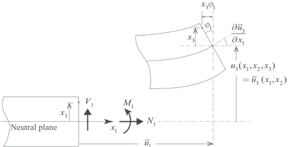
As in Figure 2, which illustrates a cross-sectional diagram viewed along the x₂-direction, the macroscopic displacement fieldsui(i=1∼3)in thick plate theory are given by

⎧⎪

⎨⎪

⎩

u₁(x₁,x₂;x₃) =u₁(x₁,x₂) −x₃𝜙1(x₁,x₂) u2(x1,x2;x3) =u2(x1,x2) −x3𝜙2(x1,x2) u3(x1,x2) =u3(x1,x2)

(1)

whereua(a=1,2)is the in-plane displacements on the neutral plane and𝜙a(a=1,2)indicates the rotation angles of the vertical sections with respect to thex1andx2axes, respectively. Additionally, Na,Ma,Va(a=1,2)in Figure 2 respectively indicate the in-plane generalized (resultant) stresses, bending moments, and transverse resultant shear stresses for the cross section. Thus, the macroscopic strain can be computed as

E=

⎧⎪

⎪⎪

⎨⎪

⎪⎪

⎩ E11

E22

E33

2E12

2E23

2E₃₁

⎫⎪

⎪⎪

⎬⎪

⎪⎪

⎭

=

⎧⎪

⎪⎪

⎪⎨

⎪⎪

⎪⎪

⎩

𝜕u₁

𝜕x1

−x₃^𝜕𝜙1

𝜕x1

𝜕u2

𝜕x₂ −x3𝜕𝜙2

𝜕x₂

0

𝜕u1

𝜕x₂ +^𝜕u2

𝜕x₁ −x3

(_𝜕𝜙

2

𝜕x₁ +^𝜕𝜙1

𝜕x₂

)

𝜕u3

𝜕x₂ −𝜙2

𝜕u₃

𝜕x1

−𝜙1

⎫⎪

⎪⎪

⎪⎬

⎪⎪

⎪⎪

⎭

=

⎧⎪

⎪⎪

⎨⎪

⎪⎪

⎩

Ẽ¹+x₃Ẽ⁴ Ẽ²+x3Ẽ⁵

̃ 0

E³+x3Ẽ⁶ Ẽ⁷ Ẽ⁸

⎫⎪

⎪⎪

⎬⎪

⎪⎪

⎭

(2)

Here,Ẽ^I (I=1∼8)is the generalized macroscopic strains, defined as Ẽ ={Ẽ¹ Ẽ² Ẽ³ Ẽ⁴ Ẽ⁵ Ẽ⁶ Ẽ⁷ Ẽ⁸}T

= {_𝜕u

1

𝜕x1

𝜕u2

𝜕x2

𝜕u2

𝜕x1

+^𝜕u1

𝜕x2

−^𝜕𝜙1

𝜕x1

−^𝜕𝜙2

𝜕x2

− (_𝜕𝜙

2

𝜕x1

+^𝜕𝜙1

𝜕x2

) _𝜕u

3

𝜕x2

−𝜙2 𝜕u3

𝜕x1

−𝜙1

}T (3)

whose deformation modes are depicted in Figure 3.

The microscopic strain𝜺is defined as the sum of the macroscopic strain and microscopic strain fluctuations, thus

𝜺=̃zẼ +𝜕yu^∗, (4)

Figure 2. Displacement fields in thick plate theory.

Figure 3. Deformation modes represented as generalize macroscopic strains.

where we have defined the following matrix expressions:

̃ z=

⎡⎢

⎢⎢

⎢⎢

⎢⎣

1 0 0 z3 0 0 0 0 0 1 0 0 z₃ 0 0 0 0 0 0 0 0 0 0 0 0 0 1 0 0 z₃ 0 0 0 0 0 0 0 −z₁∕2 1 0 0 0 0 0 0 −z₂∕2 0 1

⎤⎥

⎥⎥

⎥⎥

⎥⎦

and 𝜕yu^∗=

⎡⎢

⎢⎢

⎢⎢

⎢⎢

⎢⎣

𝜕

𝜕y1

0 0

0 ^𝜕

𝜕y₂ 0 0 0 _𝜕y^𝜕

𝜕 3

𝜕y2

𝜕

𝜕y1

0 0 ^𝜕

𝜕y3

𝜕

𝜕y2

𝜕

𝜕y₃ 0 ^𝜕

𝜕y₁

⎤⎥

⎥⎥

⎥⎥

⎥⎥

⎥⎦

⎧⎪

⎨⎪

⎩ u^∗₁ u^∗₂ u^∗

3

⎫⎪

⎬⎪

⎭

(5)

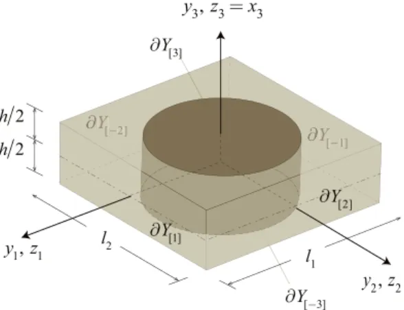
Figure 4. In-plane unit cell.

Here, two coordinate systems,y_i andzi, are used in these equations. Whereasy_iis the microscale coordinate system used for the homogenization process,ziare merely kinematic parameters used to represent the kinematics in the standard plate theory. Note thatzi is identified with the macroscale coordinate system used in formulating the macroscopic equations; see Figure 4. Moreover, matrix

̃

ztransforms the generalized macroscopic strain into a microscopic strain whose components are independent of the microscale heterogeneities. Here, components −z₁∕2 and −z₂∕2 may appear undesirable but are required for consistency with the macroscopic torsional deformations; see [25]

for a detailed explanation. Finally,𝜕yu^∗(y)is the microscopic strain fluctuation excited by microscale heterogeneities, andu^*is the corresponding displacement field that is intended to satisfy the in-plane periodic boundary conditions, or, equivalently, ‘in-plane Y-periodicity’.

Using the aforementioned expressions, we formulate the following set of governing equations for the microscopic BVP for an in-plane unit cell domain,Y=l₁l₂l₃:

⎧⎪

⎪⎨

⎪⎪

⎩

𝜕^Ty𝝈 =0 𝝈=C(

𝜺−𝜺^th) 𝜺=̃zẼ +𝜕yu^∗=𝜕yw

𝜺^th=𝛼ΔT𝝍, 𝝍= {1 1 1 0 0 0}^T u^∗∶in-plane Y-periodic

(6)

where𝝈(y)is the microscopic stress,wis the microscopic displacement, and𝜺^this the microscopic thermal strain, withΔTbeing the temperature change. Here,Cis a standard matrix for storing elastic constants, and𝛼is the coefficient of thermal expansion (CTE) used for the in-plane unit cell. With macroscopic excitations Ẽ and ΔTgiven as input data in addition to the material constants, the governing equations must be solved for the unknown fluctuating displacement fieldu^* under the in-plane periodic boundary conditions.

Conversely, generalized macroscopic stress is defined as M̃ =

∫

h∕2

−h∕2

z^T ( 1

l1l2∫

l₁∕2

−l₁∕2∫

l₂∕2

−l₂∕2

𝝈dy1dy2

) dz3=

∫

h∕2

−h∕2

z^TΣdz3 (7) wherez3 has replaced y₃, and the following definition is applied under the assumption that 𝝈 is independent ofz_i(i=1,2):

Σ(z3) = 1 A∫

l₁∕2

−l₁∕2∫

l₂∕2

−l₂∕2

𝝈(y1, y2, z3)dy1dy2 (8)

whereA = l1l2is the in-plane cross-sectional area. Here, components−z1∕2 and−z2∕2 of̃zhave disappeared inz [25]. Simultaneously, the equation relating generalized macroscopic stress and strain is recognized as

M̃ =D̃

(Ẽ − ΔTẼ^th )

=D̃Ẽ − ΔTM̃^th (9) whereD̃ is the homogenized plate stiffness matrix. Here,Ẽ^thandM̃^thare the generalized macroscopic thermal strain and stress per unit temperature change, respectively.

In this study, the components ofD̃ andM̃^thare obtained by conducting NPTs independently, each of which corresponds to the process of solving the microscopic BVP (6). Please refer to Appendix A for details concerning the NPT.

2.2. Incorporation of co-rotational formulation

In this section, the CR formulation is introduced, to enable consideration of the large rotations that occur during the in-plane homogenization analyses performed with the local coordinate system attached to each plate element.

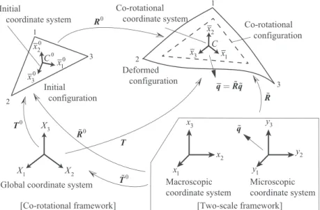
In the CR formulation, the total motion of each FE is decomposed into rigid body motion and pure deformation. For this decomposition, we define three separate configurations as illustrated in Figure 5, namely, initial, CR, and deformed configurations. Here, the CR configuration, located mid- way between the initial and deformed configurations, is a virtual configuration that undergoes rigid body motions only. Therefore, the motion from CR to deformed configurations becomes a pure defor- mation that can be either finite or infinitesimal. In this study, a linearly elastic material is assumed for the pure deformation in the CR coordinate system within the small strain framework. Under this assumption, the NPT presented in the previous section, and in Appendix A, can be conducted without any modification of the CR configuration of each element.

As depicted in Figure 5, each configuration has its own coordinate system. The local coordinate systemC-x₁x₂x₃ embedded in the CR configuration is denoted the CR coordinate system because these systems co-rotate. Here, rotation matrixR⁰is applied to rotate the initial configuration, with its coordinate systemC⁰-x⁰₁x⁰₂x⁰₃, to the CR configuration. The coordinate transformations from the global coordinate system to the initial and CR coordinate systems are then realized using transforma- tion matricesT⁰andT, respectively, so that each elemental internal force vector and tangent stiffness matrix computed for the CR configuration are transformed to the global coordinate system.

Figure 5. Configurations with global and local coordinate systems in co-rotational formulation.

The aforementioned setting is common to the CR framework but must be properly linked with the two-scale framework to accommodate the two-scale plate model with NPTs. To do this, the rela- tionship between the CR coordinate system and the microscale coordinate system for NPTs, which normally is assumed to be consistent with the macroscale coordinate system, must be defined first.

Because the orientation of an initial coordinate system is automatically generated in accordance with the numbering of element nodes in the CR formulation implementation, we first define the positional relationship between the microscale and global coordinate systems with transformation matrixT̃⁰. The transformation from the microscale to initial coordinate systems then can be rec- ognized asR̃⁰ = T⁰T̃⁰. Accordingly, we transform vectorq, defined in the microscale coordinatẽ system asq⁰=R̃⁰q̃in the initial coordinate system. Becauseq=R⁰q⁰, the transformation from the microscopic to CR coordinate systems is given by

q=R̃q̃ (10)

whereqis a vector in the CR coordinate system and the transformation matrix is defined asR̃ =R⁰R̃⁰. Thus, the computations applied to the actual elements in the present two-scale CR framework begin by evaluating the internal force vector f̃_e for each plate element in the microscale coordi- nate system produced by the generalized elastic displacement vectorp̃^e= {ũ^e, ̃𝜽^e}and temperature change, expressed as

̃f_e=k̃_ep̃^e−f̃^th_e (11)

where the element stiffness matrixk̃_eand thermal force vectorf̃^th_e are respectively defined with k̃_e=

∫ B̃^TD̃BdΩ̃ _ele (12)

̃f^th_e =

∫ ΔTB̃^TM̃^thdΩ_ele (13) Here,D̃ is the homogenized plate stiffness matrix, andB̃ is the translation matrix from the generalized elastic displacement vector into the generalized strain vector,Ẽ =B̃p̃^e.

Using the relationship in (10), we have the internal force vector in the CR coordinate system as f_e=R̃̃f_e=R̃

(k̃_ep̃^e−f̃^th_e )

=R̃k̃_e (R̃^Tp^e

)

−R̃̃f^th_e =

(R̃k̃_eR̃^T )

p^e−R̃̃f^th_e =k_ep^e−f^th_e (14) wherep^e=R̃p̃^e,k_e=R̃̃k_eR̃^Tand f^th_e =R̃̃f^th_e. Thus, the element stiffness matrix in the CR coordinate system can be computed as

ke=

∫ R̃B̃^TD̃B̃R̃^TdΩele=

∫ B^TDBdΩ̃ ele (15) where we have definedB=B̃R̃^T.

To obtain the internal force vector in the global coordinate system, we postulate that the virtual work in both the global and CR coordinate systems are conjugate, such that

𝛿d^Tf_e=𝛿p^eTf_e (16)

The generalized (virtual) elastic displacement vector in the CR framework, described in detail in Appendix B, is related to the global coordinate system as

𝛿p^e=𝚲𝛿d (17)

Thus, for any𝛿d, Equation (16) becomes

𝛿d^Tf_e=𝛿d^T𝚲^Tf_e (18)

which yields the following relationship between the internal force vectors in the global and CR coordinate systems:

f_e=𝚲^Tf_e (19)

A consistent tangent stiffness is established by linearizing this equation with respect to the general- ized total displacement vector𝛿d, with

𝛿f_e=k^e_T𝛿d (20)

wherek^e_Tis the element tangent stiffness matrix whose derivation is detailed in the literature; see, for example, [31, 33].

3. TWO-SCALE TOPOLOGY OPTIMIZATION PROBLEMS

In this section, after introducing design variables such as those used in standard or single-scale topol- ogy optimization, we present two individual two-scale topology optimization problems. Sensitivity analyses of the objective functions and the homogenized quantities are then conducted for both prob- lems. Finally, the accuracy of the derived sensitivities is verified by comparison with sensitivities evaluated through numerical differentiations.

3.1. Design variables and effective material parameters for in-plane unit cell

Assuming that the in-plane unit cell consists of two different materials and that spatial discretization with FEs is completed, we choose the volume fraction for one of the materials for FEias design variablesi, with range 0 ⩽ si ⩽ 1. Then, using a developed optimization algorithm, the material distribution of the in-plane unit cell is updated by changing values ofs_i to maximize the macro- scopic mechanical performance. In this context, the microscopic stress𝝈evaluated using the second equation of (6) is rewritten as

𝝈(s) =C( 𝜺−𝜺^th)

=C(

E⁰(s)𝜺(s) −𝛽(s)ΔT𝝍)

(21) whereE⁰is Young’s modulus,𝛽=𝛼E⁰is the coefficient of thermal stress (CTS) [34], andC=C∕E⁰ is the elasticity matrix independent ofE⁰.

Young’s modulus E⁰ and the CTS 𝛽 are then defined as functions of design variable s_i in elementi. More specifically, employing the RAMP method [34, 35], we introduce the following nonlinear interpolation functions for the effective Young’s modulus and the effective CTS, both of which vary withsi:

E⁰(s_i) = (

1− si

1+q_E⁰(1−s_i) )

E⁰_I +

( si

1+q_E⁰(1−s_i) )

E⁰_II (22)

𝛽(s_i) = (

1− s_i

1+q_𝛽(1−si) )

𝛽I+

( s_i 1+q_𝛽(1−si)

)

𝛽II (23)

whereE⁰_I and𝛽Iare the Young’s modulus and CTS of Phase I, respectively. Here,qE⁰ andq_𝛽 are penalty parameters independent of the underlying physical phenomena. The combination of these parameters in the RAMP method has been explored in depth in Reference [34], which concludes that the set ofq_E⁰ = 8 andq_𝛽 = 0 makes optimization calculations stable for thermo-mechanical optimization problems. Because the same empirical evidence was found during this study, these values are employed for the calculations in the following sections.

3.2. Optimization problems

Two two-scale topology optimization problems are now presented, one to maximize the macroscopic stiffness of a composite plate and the other to maximize the macroscopic displacements at prescribed nodes.

3.2.1. Problem I: In-plane unit cell that maximizes macroscopic stiffness. To determine an in-plane unit cell that maximizes the macroscopic overall stiffness, we formulate the following optimization problem by defining specific objective and constraint functions:

minf(s) =F^T_extU(s) (24)

subject toh(s) =

n∑elem

i=1

sivi−V0 =0 (25)

Here,U(s)is the generalized (global) macroscopic nodal displacement vector, andF_extis the gener- alized (global) macroscopic nodal (external) force vector. Also,n_elemis the total number of FEs, and v_iis the volume of elementi. The minimization of objective functionf(s)representing the macro- scopic end compliance is equivalent to maximization of the macroscopic overall stiffness in this case.

Additionally, equality constrainth(s)in Equation (25) requires the total volume of Phase 2 in the in- plane unit cell to be identical to the prescribed valueV₀. Temperature changes are not considered in this optimization problem.

3.2.2. Problem II: In-plane unit cell that maximizes specific nodal displacements. By using macro- scopic quasi-end-compliance as an objective function, we formulate an optimization problem to maximize certain nodal displacements of the macroscopic plate under thermal loading attributable toΔT, as

minf(s) =F^vTU(s) (26)

along with constraint (25). Here,Uis the generalized macroscopic nodal displacement vector, andF^v is the virtual force vector, in which only selected components ofF^v_k have non-zero values, whereas the others are zero:

U(s) = (U1,U2,· · ·,Uk,· · ·)^T (27)

F^v= (F₁^v,F^v₂,· · ·,F^v_k,· · ·)^T= (0,0,· · ·,F^v_k,0,· · ·)^T (28) 3.2.3. Optimization calculation schemes. For gradient-based topology optimization problems, two optimization algorithms, namely, the optimality criterial (OC) method [36] and the method of moving asymptotes [37], are generally used. The OC is employed for Problem I (stiffness maximization problem) because the objective function itself is a ‘monotonously increasing/decreasing function’

for any design variable and the constraint is represented by a linear function. It is indeed known that the OC method is effective to solve this kind of optimization problems and provides reliable optimization results with fast convergence. On the contrary, we apply method of moving asymptotes for Problem II because the objective function is not necessarily monotonously varying; this is a typical condition for topology optimization to maximize/minimize mean compliance of a structure subjected to thermal expansion or self-weight. With this background, the equality constraint (25) is converted to an inequality condition that must be satisfied within a small error range.

To suppress checkerboarding in optimized topologies, a particular filtering technique must be applied. In this study, the sensitivity of each element is replaced by the weighted-average of sensitivities of adjacent elements [38] as

𝜕̃f^∗(s)

𝜕si

=

∑n_elem j=1

1 v_jwijsj𝜕f^∗

𝜕s_j

∑n_elem j=1

1

v_jw_ijs_j (29)

whereiandjare element numbers. Here, we have introducedwij =exp [

−¹

2( ^rij

r⁰∕2) ]

as a weight of j for element i [39], in which rij is the distance between the centers of elements i andj, andr⁰

defines the domain of filtering. This filter has widely been utilized because of its usability, although it has no theoretical underpinning [38, 40]. Better optimization results could be obtained if we utilize theoretically proven and hence more reliable filters such as a class of ‘density filters’; see early developments in [27, 41] and more recently proposed ones in [42]. This point must be an issue to be addressed in the future.

It should also be noted that the framework of the proposed two-scale topology optimization is almost the same as that introduced by Katoet al.[12], except that microscopic analyses, or equiva- lently NPTs, must be conducted for in-plane unit cells instead of for unit cells with 3D periodicity.

Therefore, the computer implementation requires few modifications relevant to in-plane homoge- nization. In addition, the two-scale optimization algorithm itself guarantees low-computational cost because of the method of multi-scale decoupling analysis [13]. However, microscopic analyses in the iterative procedure used in this method requires more computational cost than those of [12], because constraints (A7) for NPT imply that the microscopic stiffness matrices become dense; see Refer- ence [25]. Nonetheless, computational cost required in the proposed two-scale topology optimization method is substantially smaller than that based on multi-scale coupling analysis.

3.3. Sensitivity analyses

Using the adjoint method, we now present the analytical sensitivities of the objective functions intro- duced in the aforementioned optimization problems, along with the homogenized quantities with respect to design variables_i.

3.3.1. Sensitivities of objective functions. First, the objective function in Equation (25) for Problem I is replaced with an equivalent functionf^*as follows:

f^∗(s) =F^T_extU(s) −𝝀^Tr(s) (30) where𝝀is an arbitrarily chosen adjoint vector andris the macroscopic residual vector. Here,ris intended to satisfy the equilibrium conditionr = F_ext−F_int = 0. In addition, F_int is the global macroscopic internal force vector assembled from the internal force vectorsf_e of all the elements defined in Equation (19). Differentiation of Equation (30) with respect to design variablesiyields

𝜕f^∗(s)

𝜕si

= dF^T_ext dsi

U+F^T_ext𝜕U

𝜕si

−𝝀^Tdr dsi

=F^T_ext𝜕U

𝜕s_i −𝝀^T (𝜕r

𝜕U

𝜕U

𝜕s_i + 𝜕r

𝜕s_i )

=(

F^T_ext−𝝀^TK_T)𝜕U

𝜕s_i −𝝀^T𝜕r

𝜕s_i

(31)

whereK_Tis the macroscopic global tangent stiffness matrix, which is symmetric, assembled from the element tangent stiffness matricesk^e_Tdefined in Equation (20). Here, we have assumed that the external loading is independent of the design variables so that dF^T_ext∕dsivanishes. Because the adjoint vector𝝀can accommodate arbitrary components, we can satisfy the following equation:

Fext=KT𝝀 (32)

which eliminates the first term of Equation (31). Thus, Equation (31) yields

𝜕f^∗(s)

𝜕s_i = −𝝀^T𝜕r(s)

𝜕s_i (33)

Because only the homogenized plate stiffness for the internal force vectork_ep^e in Equation (14) explicitly depend on design variablesiin𝜕r∕𝜕si, the sensitivity of𝜕r∕𝜕sican be computed as

𝜕r(s)

𝜕si

= 𝜕F^int

𝜕si

=Ae=1∫ 𝜕f_e

𝜕si

dΩ =∫ 𝚲^TB^T𝜕 ̃D

𝜕si

Bp^edΩ (34)

where Equations (15) and (19) are utilized. Note thatA_e=1indicates the assembly operator.

The sensitivity of the objective function (26) in Problem II can also be derived in a similar manner, with an adjoint vector that satisfies the following equation:

F^v =K_T𝝀 (35)

The only difference is that thermal force vectorf̃^th_e in Equation (14) is now involved such that

𝜕r(s)

𝜕si

=∫ 𝚲^TB^T (𝜕 ̃D

𝜕si

Bp^e− ΔT𝜕 ̃M^th

𝜕si

)

dΩ (36)

3.3.2. Sensitivity of homogenized plate stiffness matrix and generalized thermal strain. By multi- plying the homogenized plate stiffness matrix by the generalized macroscopic strain vector whose b-th component has a value of one while the other component values are zero, denotedẼ^b, we can compute theb-th column vector. Next, componentD_a,b is obtained via the inner product between theb-th column vector and the generalized macroscopic strain vector whosea-th component has a value of one while the other components are zero, denotedẼ^a. Thus, we have

D̃ab(s) = (Ẽ^(a)

)T

D̃Ẽ^(b) (37)

Ẽ^(a)={Ẽ¹ · · · Ẽ^a · · · Ẽ⁸}T

={

0 · · · 1 · · · 0}T

(38) Ẽ^(b)={Ẽ¹ · · · Ẽ^b · · · Ẽ⁸}T

={

0 · · · 1 · · · 0}T

(39) In view of Equations (4), (7), and (9),D̃_a,bin Equation (37) can be expressed with the microscopic strain and stress as

D̃ab(s) = 1 A

(Ẽ^(a) )T

∫_Yz^T𝝈^(b)dY

= 1

A∫_Y(𝜺^(a)−𝜕yu^∗)^T𝝈^(b)dY

= 1

A∫_Y𝜺^(a)TC𝜺^(b)dY

(40)

Here, we have utilized the microscopic equilibrium equation∫_V𝜕yu^∗T𝝈^(b)dV =0 under the condition ΔT=0. In Equation (40),𝜺^(a)and𝜺^(b)are the microscopic strain vectors obtained as solutions of the governing equation, (6), with the aforementioned generalized macroscopic strainsE^(a)andE^(b)used as data. Based on the aforementioned equations, derivatives of the components of the homogenized stiffness matrix𝜕 ̃D_ab(s_i)∕𝜕s_iare now derived as

𝜕 ̃D_ab(s)

𝜕s_i = 1

A∫_V𝜺^(a)T𝜕C

𝜕s_i𝜺^(b)dV+ 1 A∫_V𝜕𝜺^(a)

𝜕s_i

T

C𝜺^(b)dV+1

A∫_V𝜺^(a)TC𝜕𝜺^(b)

𝜕s_i dV

= 1

A∫_V𝜺^(a)T𝜕C

𝜕s_i𝜺^(b)dV

(41)

given that𝜕𝜺∕𝜕s_i=𝜕(

𝜕yu^∗)

∕𝜕s_i. Thus, the analytical sensitivity ofD̃ with respect tos_ibecomes

𝜕 ̃Dab(s)

𝜕si

= 1

A∫_V𝜺^(a)T𝜕E⁰

𝜕si

C𝜺^(b)dV (42)

The sensitivity of the generalized thermal stress can also be derived in a similar manner. With the components of the generalized thermal stress vectorM̃_a^thexpressed as

M̃^th_a(s) = (Ẽ^(a)

)T

M̃ = 1

A∫_V𝜺^(a)TC

(𝜺^(th)−𝛽C𝝍)

dV (43)

the analytical sensitivities of theacomponents of𝜕 ̃M^th(s)∕𝜕sibecome

𝜕 ̃M^th_a(s)

𝜕si

= 1 A∫V

𝜺^(a)T (𝜕E⁰

𝜕si

C𝜺^(th)− 𝜕𝛽

𝜕si

C𝝍 )

dV (44)

where𝜺^(th)is the microscopic strain obtained as a solution for governing Equation (6), with the data expressed in (A6) that uses NPTs to evaluate the generalize macroscopic thermal strain.

4. NUMERICAL EXAMPLES

In this section, we present several numerical examples for Problems I and II, which are defined in the previous section, to demonstrate the potential of the proposed two-scale topology optimization method for the design of composite plates with in-plane periodicity.

4.1. Problem I: Maximization of macroscopic stiffness

Let us determine a single optimal topology of an in-plane unit cell that maximizes the macroscopic stiffness of the overall composite plate structure. Because the proposed two-scale topology opti- mization method is based on in-plane homogenization, the asymmetry of the material distribution in an in-plane unit cell activates the coupling between the transverse shear and the in-plane/out- of-plane deformations, as demonstrated in Reference [25]. Additionally, because large rotations of the macroscopic plate are allowed, the optimal topology is expected to depend on the amount of macroscopic deformation. To illustrate the unique features of the proposed method, we define the macroscopic problem illustrated in Figure 6 and conduct two cases with different loading parame- ters,𝜇=1.0×10⁵and𝜇=8.0×10⁸, which correspond to small and large rotations, respectively.

We note that the macrostructure can be classified as a thick plate because the ratio of the thickness to the axial length is 0.1. Bending about thex2-axis and the transverse shear in thex1x3-plane is there- fore predominant compared with other deformations. In this numerical example, the in-plane unit

Figure 6. Finite element mesh and boundary conditions for Problem I.

cell is cubic and composed of a single material whose Young’s modulus and Poisson’s ratio are set at 1.0×10¹⁰and 0.3, respectively, and its FE model is composed of 16×16×16 3D cubic solid ele- ments that have 14,739 degrees-of-freedom (DOFs). However, the macrostructure is composed of 1800 three-node triangular flat-shell elements and has 5766 DOFs. Moreover, the radius of filtering presented in Equation (29) is set atr₀=0.01 that is one-tenth of one side of the in-plane unit cell.

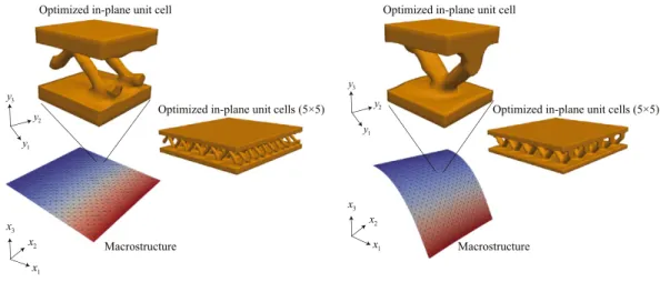
The obtained optimal topologies for the two loading cases are shown in Figure 7. Here, the design variables are converted as elemental values to nodal values so that smooth iso-surfaces are visualized by standard visualization software. In both of the obtained in-plane unit cell topologies, material is distributed in the upper and bottom portions, causing the composite plate resist bending deforma- tions, and diagonal members in thex₁x₃-plane are formed that create resistance to transverse shear deformations. At first glance, they are similar to each other in terms of topological feature. How- ever, differences in certain components of the homogenized plate stiffness matrices obtained from the optimal in-plane unit cells, as listed in Table I, can be recognized. Here, the upper indices of D̃^SandD̃^Lindicate those obtained for the small and large rotation cases, respectively. In particular, their(1,4)components, which indicate the degree of coupling between the in-plane strainẼ1 and curvatureẼ4, differ substantially. Furthermore, there is a noticeable difference between the(1,8) components, which reflect the coupling between the membrane forceM̃1 and the transverse shear strainẼ8. More specifically, these components in the large rotation case have larger values than those of the small rotation case. This is probably because that the bending and transverse shear deforma- tions caused by the membrane force, which are increased in the plate subjected to large rotation, must be suppressed. Figure 8 shows the convergence history of the normalized objective functions with respect to the number of iterations for these optimization calculations, both of which exhibit the convergences with approximately 500 iterations.

Figure 7. Optimal topologies for Problem I.

Table I. Selected stiffnesses of optimal in-plane unit cell.

Components(a,b) D̃^La,b D̃^Sa,b

D̃_1,1[N/m] 4.07×10⁸ 4.32×10⁸ D̃1,4[N] −1.28×10⁶ −2.75×10⁴ D̃4,4[N·m] 6.72×10⁵ 7.07×10⁵ D̃_1,8[N] −1.28×10⁶ −6.66×10⁵ D̃8,8[N/m] 1.44×10⁷ 1.14×10⁷

Figure 8. Iteration history of the normalized objective function.

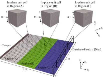
Figure 9. Finite element mesh with three regions to assign separate in-plane unit cells for Problem I.

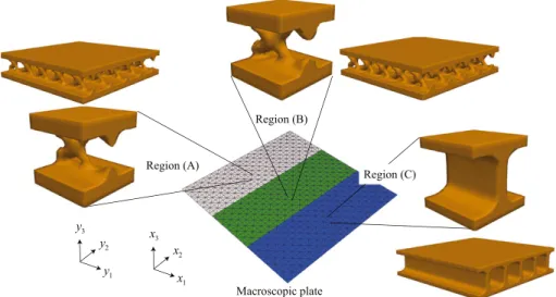
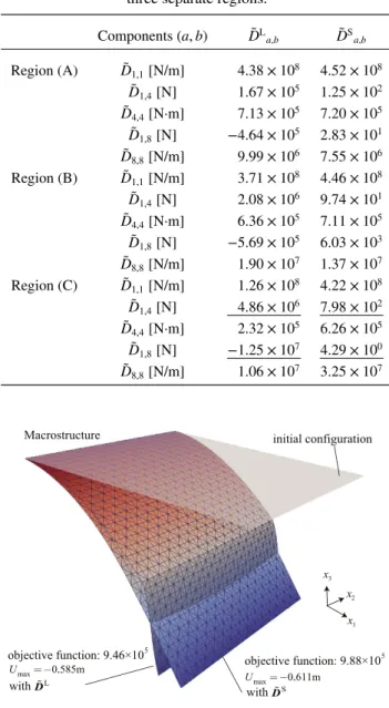
To confirm the aforementioned points, we considered a macrostructure in which in-plane unit cells were separately assigned to three specified regions, designated Regions (A), (B), and (C), as shown in Figure 9, and solved the same set of optimization problems as before. The obtained optimal topologies for the cases of small and large rotation are presented in Figures 10 and 11, respectively.

As these figures illustrate, the optimized topologies of the in-plane unit cells in Regions (A) and (B) are similar for both rotation cases, but those of the in-plane unit cells in Region (C) are markedly different. Whereas the Region (C) optimal topology obtained for the small rotation case has a sim- ple wall member that resists the transverse shear deformation, that of the large rotation case has a more complex and asymmetric structure with respect to both they₁y₂ andy₂y₃ planes. This asym- metric material distribution acts to couple the components of the homogenized plate stiffness matrix.

Indeed, as the data in Table II indicate, the in-plane unit cell in Region (C) yields relatively large values in the components representing the coupling of the in-plane membrane strainẼ1 for both bending and transverse shear deformations,Ẽ₄andẼ₈. Thus, the bending and transverse shear defor- mations induced by the in-plane membrane stress seems to effectively increase the overall stiffness of the macroscopic plate in this case for large rotation. To confirm the effectiveness of this increase, we conducted two separate macroscopic analyses with loading parameter𝜇 =8.0×10⁸ (the pre- vious large rotation setting) using the homogenized plate stiffness matricesD̃^LandD̃^Sobtained for

Figure 10. Three optimal topologies under small rotation setting.

Figure 11. Three optimal topologies under large rotation setting.

Regions (A), (B), and (C). The results appear in Figure 12 and demonstrate that the obtained opti- mal topologies are physically reasonable, because the deflection of the macroscopic plate withD̃^L is smaller than that withD̃^S.

4.2. Problem II: Maximization of nodal displacement vector components

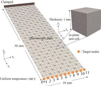
We now perform analyses for an optimal topology of an in-plane unit cell that maximizes selected macroscopic nodal displacements to enable adjustment of the macroscopic motion of a composite plate. The FE model of the macroscopic plate is shown in Figure 13, in which target nodes are specified. This model is composed of 600 three-node triangular flat-shell elements and has 2046 DOFs (341 nodes), whereas the FE model of the in-place unit-cell is the same as that in Problem I.

In the numerical examples below, the following two cases have virtual force vectors set for the nodes of interest:

Table II. Selected stiffnesses of optimal in-plane unit cells in three separate regions.

Components(a,b) D̃^La,b D̃^Sa,b

Region (A) D̃1,1[N/m] 4.38×10⁸ 4.52×10⁸ D̃1,4[N] 1.67×10⁵ 1.25×10² D̃4,4[N·m] 7.13×10⁵ 7.20×10⁵ D̃_1,8[N] −4.64×10⁵ 2.83×10¹ D̃8,8[N/m] 9.99×10⁶ 7.55×10⁶ Region (B) D̃_1,1[N/m] 3.71×10⁸ 4.46×10⁸ D̃1,4[N] 2.08×10⁶ 9.74×10¹ D̃4,4[N·m] 6.36×10⁵ 7.11×10⁵ D̃_1,8[N] −5.69×10⁵ 6.03×10³ D̃8,8[N/m] 1.90×10⁷ 1.37×10⁷ Region (C) D̃_1,1[N/m] 1.26×10⁸ 4.22×10⁸ D̃1,4[N] 4.86×10⁶ 7.98×10² D̃_4,4[N·m] 2.32×10⁵ 6.26×10⁵ D̃1,8[N] −1.25×10⁷ 4.29×10⁰ D̃8,8[N/m] 1.06×10⁷ 3.25×10⁷

Figure 12. Results withD̃^LandD̃^Sunder large rotation condition.

Case 1:F^v1=

{−1 (k=1,· · ·,11 and only z3 direction)

0 (otherwise) (45)

Case 2:F^v2=

⎧⎪

⎨⎪

⎩

1 (k=1,· · ·,3 and only z₃ direction)

−1 (k=8,· · ·,11 and only z₃ direction) 0 (otherwise)

(46)

The FE model of the in-plane unit cell, composed of two different materials, is also depicted in Figure 14. To visualize the effect of thermal deformations, we consider two patterns of material combinations for Case 1. Patterns A and B have the material constants listed in Tables III and IV, respectively. Here, both Young’s moduli and CTEs for the constituents are different for Pattern A, whereas only CTEs are different for Pattern B.