富山大学工学部紀要
第55巻
Bulletin of
Faculty of Engineering Toyama University
Vol. 55
2 0 0 4
日 次
1. A New Method to Solve the Constraint Satisfaction Problem Using the Hopfield Neural Network
…Weidong Sun, Hiroki Tamura, Zheng Tang, Masahiro Ishii… 1
2. 自己フィードバッグを考慮したニューラルネットワークによる四色問題のー解法
- 孫 鬼東, 田村 宏樹, 唐 政, 石井 雅博 ・
3. 研究業績一覧(2002年11月から2003年12月)
電気電子システム工学科 ... 15
知能情報工学科 …・... 24
機械知能システム工学科 ....・H・-…・・・・・・・・・・・・・・・・・・・・・・・・・・・・・・・・・・・・・・・・・・・・・・・・・・・・・・・・・・・・・・・・・・・・・ 34
物質生命システム工学科 …・…・... 44
4. 2003年度修士論文題名一覧 …...・H・-………・…・…....・H・..…...・H・-………...・H・-…… 57
5. 2003年度博士論文概要一覧 …...・H・..…... 67
Using the Hopfield Neural Network
Wei-Dong SUNt, Hiroki TAMURAt, Zheng TANGt, and Masahiro ISHIIt,
SUMMARY
The constraint satisfaction problem is constituted by several condition formulas, which makes it difficult to be solved. In this paper, using the Hopfield neural network, a new method is pro
posed to solve the constraint satisfaction problem by simplifying its condition formula. In this method, all restriction conditions of a constraint satisfaction problem are divided into two restrictions:
restriction I and restriction II. In processing step, restriction II is satisfied by setting its value to be 0 and the value of restriction I is always made on the decreasing direction. The optimum so-
lution could be obtained when the values of energy, restriction I and restriction II become 0 at the same time. To verify the valid
ity of the proposed method, we apply it to two typical constraint satisfaction problems: N-queens problem and four-coloring prob
lem. The simulation results show that the optimum solution can be obtained in high speed and high convergence rate. Moreover, compared with other methods, the proposed method is better than other methods.
key words: Constraint satisfaction problem, Combinatorial op
timization problem, Hopfield neural network, N-queens problem, Four-coloring problem
1. Introduction
A constraint satisfaction problem is a problem to find a consistent assignment of values to variables. It is one kind of the combinatorial optimization problem. A number of commonly encountered problems in mathe
matics, computer science, molecular biology, manage
ment science, seismology, communications, and opera
tion research belong to a class of combinatorial opti
mization problems [1]. The combinatorial optimization problem is a very difficult problem, it could take dozens of years to obtain one optimum solution even if the lat
est supercomputer is used [2] [3].
The idea of using neural network to provide solution originated in 1985 when Hopfield and Tank demon
strated that the traveling salesman problem could be solved using the Hopfield neural network [4] [5]. Since Hopfield and Tank's work [4] [5] , there has been grow
ing interest in the Hopfield neural network because of its advantages over other approaches for solving opti
mization problems. The work by Wilson and Pawley [6]
showed that the Hopfield neural network often failed to converge to valid solutions. Takefuji et al. [7] [8] modi
fied the motion equation in order to guarantee the lo- tThe authors are with the Faculty of Engineering, Toyama University; Gofuku 3190,Toyama city, JAPAN.
[email protected], [email protected]
cal minimum convergence. However, with the Hopfield neural network, the state of system is forced to converge to a local minimum. In other words, the neural network cannot always find the optimum solution. Therefore, several neuron models and heuristics such as hysteresis binary neuron model [9] , neuron filter [20], the hill
climbing term and omega function [10] , Lagrange re
laxation [11] and pots spin [12] have been proposed to improve the performance of the network. Despite the improvement of the performance of the Hopfield neural network over the past decade, this model still has some basic problems [13][14].
A constraint satisfaction problem has several con
straint conditions, and this makes it difficult to be solved. In this paper we propose a new method to solve the constraint satisfaction problem using the Hopfield neural network. In this method, all the restriction con
ditions of a constraint satisfaction problem are divided into two restrictions: restriction I and restriction II. In processing step, restriction II is satisfied by setting its value to be 0 and the value of restriction I is always made on the decreasing direction. The optimum solu
tion could be obtained when the values of energy, re
striction I and restriction II become 0 at the same time ..
To verify the validity of the proposed method, we ap
ply it to two typical constraint satisfaction problems:
N-queens problem and four-coloring problem. The sim
ulation results show that the optimum solution can be obtained in high speed and high convergence rate.
Moreover, the comparison results show that the pro
posed method is better than other methods.
The rest of this paper is organized as follows. In sec
tion 2, we briefly introduce the Hopfield neural network and its relevant components for constraint satisfaction problems. Section 3 presents the details of the pro
posed method and its formulization method. , The sim
ulation results of testing the proposed method in real constraint satisfaction problems are described in sec
tion 4 for N-queens problem and in section 5 for four
coloring problem. Finally, the paper is concluded with general comments concerning the proposed method and its effectiveness to constraint satisfaction problems ..
2. The Hopfield Neural Network for Con
straint Satisfaction Problem
In this section, we briefly introduce the Hopfield neu-
- 1-
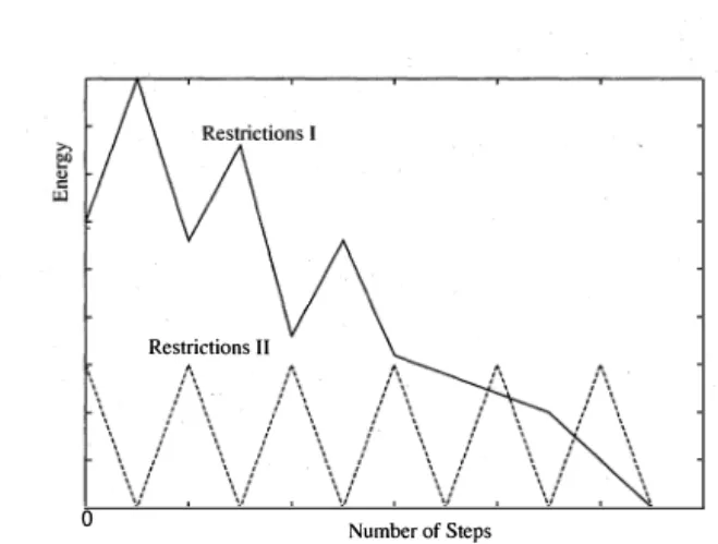
Restrictions II
\/\/\}\;/' \/ /\.,
0 Number of Steps
Fig. 1 The conceptual figure of the proposed method.
ral network and its relevant components for constraint satisfaction problems.
The Hopfield neural network for constraint satisfac
tion problems consists of two elements named neuron unit and motion equation. The neuron unit is a col
lection of simple processing elements called neurons.
Each· neuron has an input potential Ui and an output potential V;. The dynamic behavior of the network is described by the following motion equation with a par
tial derivation term of the energy function (E) and a
decay term with a time constant T [4][5].
8E(V1, V2, · · ·, VN)
8V; (1)
Takefuji et al. showed that the decay term increases the energy function under some conditions [8]. They modified the motion equation in order to guarantee the local minimum convergence.
8E(V1, v2, · · ·, vN)
8V; (2)
To compute the input potential of neurons, the time
idependent method is used in which the input potential of neurons at timet+ 1 depends on the value at time t [8].
(3) The output is updated from Ui using a non-linear function called neuron model. For example, according to the McCulloch-Pitts binary neuron model [30] , it can be obtained:
{ 1 if ui > o
Vi = 0 otherwise (4)
Each neuron updates its input potential according to the computation rule (Eq.(3)) and sends its out
put state in response to the input according to the in- put/output function (Eq.(4)). .
3. The Proposed Method to Solve Constraint Satisfaction Problem Using the Hopfield Neural Network
In this section, we describe a new method to solve con
straint satisfaction problem using the Hopfield neural network. Note that·the process in the Hopfield neural network is sequential.
3.1 Simplification of Constraint Satisfaction Problem A constraint satisfaction problem usually consists of several restriction condition formulas. In the proposed method, we classify these restriction condition formulas into two kinds: restrictions I and restrictions II . The conceptual figure of this proposed method is shown in Fig.l. Restriction I always is carried out in the de
creasing direction; restriction II are satisfied by setting its value to be 0 in processing step, in other words, if a certain value of restriction II increases , only the same quantity will decrease, and it returns to 0 surely. The optimum solution can be calculated when the values of both restrictions become 0. State change is sequen
tially performed for every neuron. If each neuron is in the state of satisfying restrictions, it can be stabilized in the state, on the contrary, it becomes unstable if it is in the state where it does not satisfy the restrictions.
Although the constraint satisfaction problem is in the tendency to become complicated since it consists of sev
eral condition formulas, if some condition formulas are satisfied in the processing, the problem will be simpli
fied and it will become easy to draw a solution. More
over, the procedure at the time of drawing the optimum solution by becoming a unary formula decreases, and it is thought that it becomes possible to draw the opti
mum solution in a short time.
3.2 Formulization for Restrictions I and II
As discussed above, the formula of a constraint sat
isfaction problem consists of two restriction condition:
restriction I and restriction II in the proposed method.
Next, we give the mathematic description for the pro
posed method.
[1] For a certain neuron (i) in time (t), the value of restriction I is assumed to be aij ( t), of restriction
II to be bik(t). Therefore, the input of neuron (i)
can be described as:
Ui ( t + 1) = restriction I + restriction I I
= aij(t) + bik(t) (5)
[2] In time (t), the energy function is assumed to be L;!1 Pj(t) for restriction I , '2:;�1 Qk(t) for
restriction II, and, Pj(t) = L;�=l aij(t), Qk(t) =
-2-
L:�=l bik(t). So, the energy function of network can be given by
M M'
E = 2:Pj(t) + LQk(t)
j=l k=l (6)
Here, Lis the number of neurons, (1, 2, · · · ,i, · · · ,L);M,
neurons number of restriction I (1, 2, · · ·, j, · · ·, M) ; M', neurons number of restriction II (1, 2, · · ·, k, · · ·, M').
Thus, according to the definition above, the following conditions will be satisfied for restrictions I and II in the proposed method.
[Restriction I ] Restrictions I is formulized as fol
lowing.
M M
LPi(t+a) - LPi(t)::::; 0
j=l j=l (7)
This formula makes the energy function always go in the reduction direction. However, t +a is the
time when the processing in the Hopfield neural network is sufficient in time t.
(Restriction ll ] Restrictions II is formulized as fol
lowing.
(8) When a step of processing is carried out about neu
ron (i), this formula presents that the value of re
strictions II at· time t + 1 is the same as that at time t, or less than it. Even if bik(t) of a neuron increases temporarily according to the conditions of restrictions I , or the conditions of the restric
tions II of other neurons, while carrying out one loop, it returns to the state of I:k=l QkM' (t) = 0
again. Therefore, it is not necessary to formulize like restriction I so that the energy function may be made to go in the reduction direction.
3.3 Algorithms
The following procedure describes the algorithms for solving constraint satisfaction problems based on the proposed method. Note that t is the step number and
Llimit is maximum number of iteration step.
Step 1. Setteing Parameters.
(a) Set t = 0, D.t = 1, and set Llimit and other parameters.
(b) Randomize the initial value of Ui (0) for i =
1, 2, ···, N.
(c) evaluate the values of 1/i(O) according to Equ.(4).
Step 2. Calculating Network Energy.
for t = 1 to Llimit, do:
(a) initialize Ui = O, fori = 1, 2, · · ·, N.
(b) Update the Ui(t + 1) and 1/i(t + 1) for i
1, 2, ···, N.
(c) Calculate the energy E according to Equ.(6).
(d) Check system energy. If E = 0 (the optimum solution can be obtained) , end the procedure.
4. Application to N-queens Problem
In this section, the proposed method is applied to one of the optimization problems: N-queens problem.
4.1 About N-queens Problem
In 1992, Takefuji presented a neural network .for· N
queens problem with the hysteresis binary neuron model [31]. Mandziuk and Macukow presented a neu
ral network using the continuous sigmoid neuron model [28]. In 1995, Mandziuk improved their neural network by using the binary neuron model [29]. In 1994, Ohta
et al. presented the neural network using the binary neuron model with the negative self-feedback [32]. In 1997, Takenaka et al. presented the neural network us
ing the maximum neuron model with the competition resolution method [21].
N-queens problem is the problem to assign N queens with no collision in N x N chess board. Queen is the piece used in chess. Queen moves for vertical, horizon
. tal and diagonal freely. One of the optimum solution of 5 queens problem is shown in Fig.2. To express the problem with neurons, we transform Fig.2 to expres
sion with 5 x 5 neurons as shown in Fig.3. The output of the neuron corresponds to an existence of a queen.
When a queen is placed, an output of the neuron is 1.
An output where no queen is placed is 0.
4.2 The Motion Equation and Energy Function The motion equation for the ijth neuron is given by:
Uij ( t + 1) = ( restriction I + restriction I I )
= -A (t Vik -1) -A (t Vki - 1)
k=l k=l
-B L Vi-k,j-k
l<::,_i-k,j-k<::,_N(k#-0)
-B l<::,_i-k,j+k<::,.N(k#-0) L Vi-k,j+k
+1/ij(t) (9)
where, A, Bare positive coefficients. In equation (9), the first term means the constraint that only on queen must be placed on row; the second term, on column; the third term, on lower right diagonal; the fourth term, on lower left diagonal. Among them, the first, second terms are corresponding to resticiton I , and the third, fourth terms are corresponding to restriction II . The
-3-
Fig. 2 An example of N-queens problem for N=5.
0 0 1 0 0
1 0 0 0 0
0 0 0 1 0
0 1 0 0 0
0 0 0 0 1
Fig. 3 Example of 5 x 5 neurons' configuration.
fifth term expresses whether there is a queen or not before updating the neuron state.
According to the Uij from the equation (9) , the value of Vii is defined by
if Uii > 0 otherwise The energy function is given by
(10)
N N { (
)}
+ B L L Vij L Vi-k,i+k
i=l j=l l�i-k,i+k�N(k#O)
According to equation (11), the first term becomes zero if one queen is placed in every row. The sec
ond term becomes zero if one queen is placed in every column and the third, fourth term become zero if no more than one queen is placed on any diagonal line.
In overall, the values of the energy function always be
come positive or 0, and it tends to increase if all con�
straints are not fulfilled. Therefore, if the neuron state is changed along the decreasing direction of energy func
tion, it is possible that the energy becomes zero. This is the optimization solution when the energy becomes zero.
4.3 Simulation Results
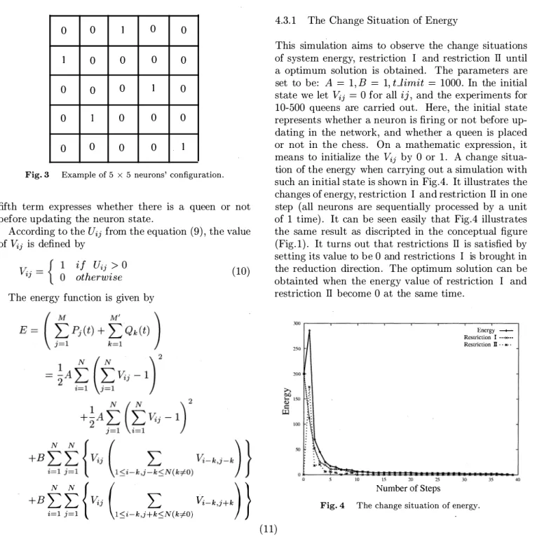
4.3.1 The Change Situation of Energy
This simulation aims to observe the change situations of system energy, restriction I and restriction Il until a optimum solution is obtained. The parameters are set to be: A = 1, B = 1, Uimit = 1000. In the initial state we let Vii = 0 for all ij, and the experiments for 10-500 queens are carried out. Here, the initial state represents whether a neuron is firing or not before up
dating in the network, and whether a queen is placed or not in the chess. On a mathematic expression, it means to initialize the Vii by 0 or 1. A change situa
tion of the energy when carrying out a simulation with such an initial state is shown in Fig.4. It illustrates the changes of energy, restriction I and restriction Il in one step (all neurons are sequentially processed by a unit of 1 time). It can be seen easily that Fig.4 illustrates the same result as discripted in the conceptual figure (Fig.1). It turns out that restrictions Il is satisfied by setting its value to be 0 and restrictions I is brought in the reduction direction. The optimum solution can be obtainted when the energy value of restriction I and restriction Il become 0 at the same time.
250
200
(11)
Number of Steps
Energy -+
Restriction I ···»··
Restriction D · · • ·
Fig. 4 The change situation of energy.
- 4 -
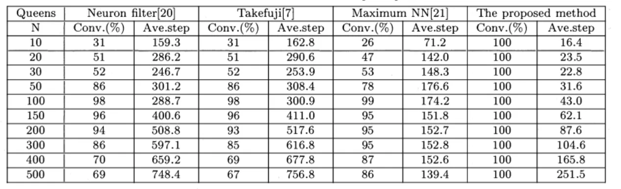
Table 1 Simulation results of N-queen problems.
Queens Neuron filter[20] Takefuji[7] Maximum NN[21] The proposed method N Conv.(%) Ave.step Conv.(%) Ave.step Conv.(%) Ave.step Conv.(%) Ave.step
10 31 159.3 31 162.8
20 51 286.2 51 290.6
30 52 246.7 52 253.9
50 86 301.2 86 308.4
100 98 288.7 98 300.9
150 96 400.6 96 411.0
200 94 508.8 93 517.6
300 86 597.1 85 616.8
400 70 659.2 69 677.8
500 69 748.4 67 756.8
4.3.2 The Result of Comparison with Other Methods This simulation aims at evaluating the validity and ef
fectivity of the proposed method by comparing with the other methods. The other methods include neuron fil
ter [20] , Takefuji method [7] and Maximum NN method [21].
In this simulation, the parameters are set to be:
A = 1, B = 1, Uimit = 1000. 100 simulations runs with different initial states are preformed for 10-500 queens.
We use the convergence rate and the number of aver
age steps of each solution method for comparison. Here, the number of average steps is the average value of the number of steps required for the convergence. The con
vergence rate expresses the average convergence times on the optimum solution during 100 trial. The simula
tion results are shown in Table 1, where the convergence rate and the average number of steps required for the convergence are summarized.
As shown in Table 1, the convergence rate in the pro
posed method is all 100% , but, in the other methods they are not so well. Furthermore, the required average steps for the proposed method are much less than the other methods. For example when N =100, the average steps are 288.7, 300.9 and 174.2 for Neuron filter [20] , Takefuji [7] and Maximum NN [21] , respectively, but the proposed needs only 43 steps for the 100% conver
gence rate. It demonstrates that the proposed method increases the convergence rate and reduces the aver
age steps compared with the other methods. That is to say, the proposed method performs better than the other methods.
5 . .Application to Four-Coloring Problem
5.1 About Four-Coloring Problem
A mapmaker colors adjacent countries with different colors so that they may be easily distinguished. This is not a problem as long as one has a large number of col
ors. However, it is more difficult with a constraint that one must use the minimum number of colors required for a given map. It is still easy to color a map with a
26 71.2 100 16.4
47 142.0 100 23.5
53 148.3 100 22.8
78 176.6 100 31.6
99 174.2 100 43.0
95 151.8 100 62.1
95 152.7 100 87.6
95 152.8 100 104.6
87 152.6 100 165.8
86 139.4 100 251.5
small number of regions. In the early 1850's, Francis Guthrie was interested in this problem, and he brought it to the attention of Augustus De Morgan. Since then many mathematicians, including Arthur Kempe, Pe
ter Tait, Percy Heawood, and others tried to prove the problem that any planar simple graph can be col
ored with four colors. A four-coloring problem is de
fined that one wants to color the regions of a map in such a way that no two adjacent regions (that is, re
gions sharing some common boundary) are of the same color. In August 1976, Appel and Haken presented their work to members of the American Mathematical Society [24]. They showed a computer-aided proof of the four-coloring problem. However, their coloring was based on the sequential method so that it took many hours to solve a large problem. Their computation time may be proportional to O(x2) where x is the number of the regions. Moreover, few parallel algorithms have been reported. Dahl [25] , Moopenn et al. [26] , and Thakoor et al. [27] have presented the first neural net
work for map K-colorability problems.
Fig. 5 An example of 7-region map.
I [�]
Z2 0 I 0 0
;g 3 0 0 I 0
.!a 4 0 0 0 I
96 0 5 0 0 I 0 0 I 0
7 I 0 0 0
1 234 567
I 0100100
2 I 0 I I I 0 0 3 0101 -001 4 0 I I 0 I I I
5 1 101000 6 0001101 7 0011010 Fig. 6 Neural representation of the 7-region map.
In order to map the four-coloring problem to the Hop
field neural network, a x x 4 two dimensional neural
-5-
array is needed, where x is the number of regions to be colored, and a single region requires four neurons for the single-color assignment. 7-region map are colored by four colors as shown in Fig.5. If red, yellow, blue and green are represented respectively by 1000, 0100, 0010 and 0001, the neural representation for the problem is given in Fig.6, where a 7 x 4 neural array is used.
Fig.6 also shows the 7 x 7 adjacency matrix D of the
seven-region map, which gives the boundary informa
tion between regions, where Dxy = 1.
5.2 The Motion Equation and Energy Function According to the four-coloring problem constraint con
ditions, we can obtain the motion equation for c neuron as
Uxc(t + 1) = (restriction I+ restriction II)
4 N
= -A(LVxk - 1) -BLDxyVyc
k=1 y=1
+Vxc(t) + dAxc (12)
where, A and B are positive constants, D is the adja
cency matrix, and Vxk is the output of kth neuron in the x region.
And depending upon the U,c, the Vxc can be deter
mined by
(Uxc > 0)
(Uxc :S: 0) (13)
In the equation (12) , the first term represents the row constraint in the neural array, which forces one region to be colored by one and only one color. It corresponds to restriction I in this paper. In the case that no color neuron is firing, 2::!=1 Vxk = 0, then -(2::!=1 Vxk -1) = + 1. It suggests that the value of U is changed on the positive direction. That is, V is drawn towards firing direction. In the case that only one color neuron is firing, 2::!=1 Vxk = 1, then -(2::!=1 Vxk - 1) = 0. It
suggests there is no change in U. Similarly, in the case that two or over two color neurons are firing, the value of U is changed in the negative direction. That is, V is
drawn towards non-firing direction.
The second term represents the same color neuron cannot be arranged in the adjacent regions. It corre
sponds the restriction II in this paper. Dxy Vyc becomes
+ 1 only in the case that the same color neuron is firing in the two adjacent regions x and y. This is because
Dxy = 0 if region x, y are not adjacent regions and
Vyc=O if the same color neurons are colored. Thus, it can be said that the second term is the sum of firing c neuron in the region adjoined with x region. Since -B
is multiplied to this sum, the more this sum is, the more V is drawn towards non-firing direction eventually.
The third term represents the color neuron state be
fore updating. In addition, since state change in the
proposed method is sequentially performed for every neuron, the value of Vxc at time (t) and time (t + 1) is
intermingled.
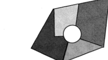
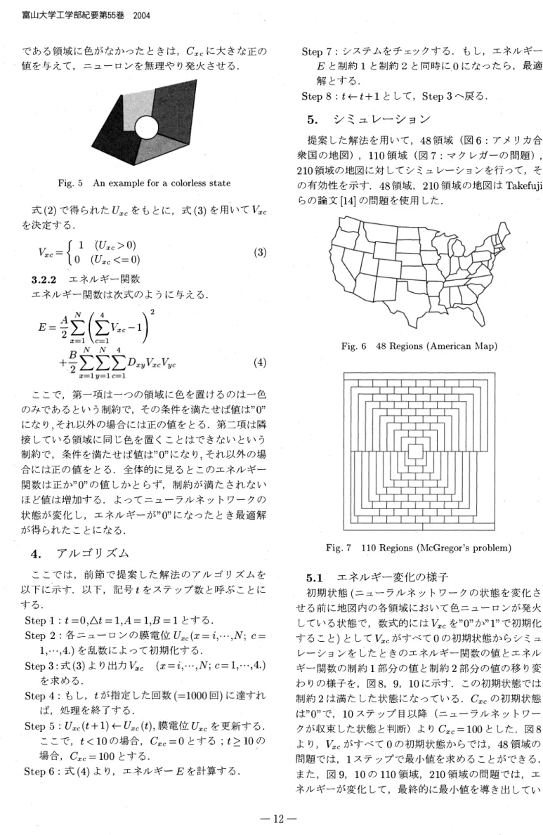
The fourth clause dAxc, which is a special term, has the motion to fire a neuron of some region (the round region of middle in Fig. 7) forcibly when surrounding of this region is colored by all four colors as shown in Fig. 7, and it is impossible to also place all the color. That is, when there is no color in the region in the convergent state, the neural network gives a positive big value to
dAxc, and make a neuron to fire forcibly.
Fig. 7 An example for a colorless state.
The energy function which arranged in the four color problem is given by the following formula using the en
ergy function of the Hopfield neural network.
E =
1 N N 4
+2BLLLDxyVxYyc (14)
x=1y=1c=1
The first term is the constraint that a region is col
ored by one and only one color. If the constraint is ful
filled, the value of the first term becomes 0, otherwise, positive value. The second term is the constraint that adjoined region cannot be colored by the same color.
If the constraint is satisfied, the value of the first term becomes 0, otherwise, positive value. On the whole, the energy function takes only positive value or 0, and its value can increase if restrictions are not satisfied.
Therefore, the energy function of the Hopfield neural network can be changed on the decreasing direction if restrictions are satisfied. When the values of two re
strictions become 0, the value of the energy becomes 0, too. Thus, the optimum solution can be obtained.
5.3 Simulation Results
In this section, we apply the proposed method to the four-coloring problem. Simulations are performed on three kinds of maps: 48 regions (American Map) , 110 regions, and 210 regions. The parameters are set to be:
A = 1, B = 1, Llimit = 1000.
-6-
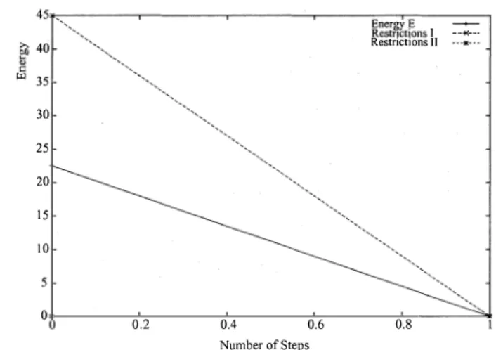
30 25 20 15 10
Fig.8
0.2 0.4 0.6
Number of Steps
EnergyE -
Restti.ctions I --*-
Restrictions II
0.8
The change situation of energy ( 48 Regions).
IOrr--�----r---�--�----�---.�ne���E�----.
Restnctions I --•-
2
00
Fig. 9
2
Fig.lO
Restrictions II ---•-- ·
/\ /\
�-i \_:;.'
10 15 20 25
Numebr of Steps
The change situation of energy (110 Regions).
4 6 10
Number of Steps 12
EnergyE - Restrictions I --*-
Restrictions II ---•---
�----� r
\,!'\/'
14
The change situation of energy (210 Regions).
5.3. 1 The Change Situation of the Energy
40
This simulation aims to observe the change situations of system energy, restriction I and restriction II until a optimum solution is obtained. First, in the initial state
we let V.,c =0, the change state of energy, restriction
I and restriction II are illustrated in Fig.8, Fig.9 and Fig. 10, respectively. The initial value of dA.,c is set to be 0, and after 10 steps (It is judged as the convergence state of the Hopfield neural network.) , it is. set to be 100.
As shown in Fig.8, the minimum value can be obtained in 1 step for the 48 regions. Fig.8, Fig.9 and Fig.10 illustrate that restriction I is drawn on the decreasing direction and the restriction II is always satisfied until the convergence state of the Hopfield neural network is obtained. It turns out that this is in agreement with that explained in Section 3 (see Fig. 1 ) .
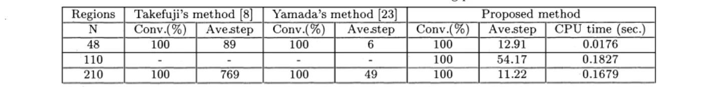
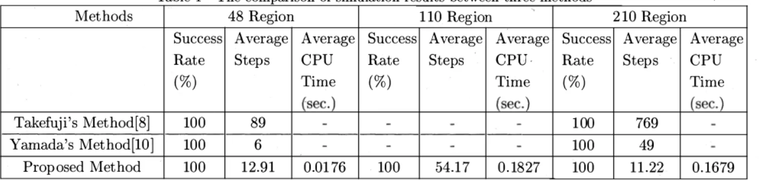
5.3.2 The Comparison with Other Methods
Next, in order to compare the proposed method with the other methods, the simulations are performed 100 times from different initial state. As ·examples, the other methods include Takefuji method [8] and Yamada method [23] . The datas of Takefuji method and Ya
mada method used in this paper are from the data car
ried by the paper [23] . The regions that can be com
pared are the map of 48 regions and 210 regions, and we use the convergence rate and the number of average steps of each solution method for comparison. Here, the number of average steps is the average value of the number of steps required for the convergence. The con
vergence rate expresses the average convergence times on the optimum solution during 100 trial. The simula
tion results are shown in Table 2.
Table 2 shows that the 100% convergence rate can be obtained in all solution methods. It turns out that the minimum value can be calculated with the fewest num
ber of steps for the 48 regions map. However, as shown in Fig.8, the minimum value can also be calculated at only one step by the proposed method depending on the initial state of neurons. By the simulation result of 210 regions, the minimum value can be calculated with the fewest number of steps. It depicts that the proposed method is better than the other methods.
Moreover, the average CPU time at the time of con
vergence obtained by the proposed method is shown in Table 2, too. It suggests that the four-coloring prob
lem with which it dealt in this paper can be solved in several seconds.
In addition, the computer to perform the simulations in this paper is CPU: Pentium ill 800Hz; OS: Winodws 2000; and the compiler is performed in the environment of VC++6.0.
6 . Conclutions
In this paper, we proposed a new method to solve the constraint satisfaction problems using the Hopfield neu
ral network. In this method, all the restriction condi
tions of a constraint satisfaction problem are divided into two restrictions: restriction I and restriction II.
- 7-
Table 2 Simulation results of four-coloring problems.
Regions Takefuji's method [8] Yamada's method [23] Proposed method N Conv.(%) Ave.step Conv.(%)
48 100 89 100
llO - - -
210 100 769 100
In processing step, restriction II is satisfied by setting its value to be 0 and the value of restriction I is al
ways made on the decreasing direction. The optimum solution could be obtained when the values of energy, restriction I and restriction II become 0 at the same time. As two typical examples of constraint satisfac
tion problems, the proposed method was demonstrated by simulating the N-queens problem and four-coloring problem. The simulation results showed that the pro
posed method could increase the convergence rate and reduce the average steps and perform better than the other methods.
References
[1] R. Garey and S. Johnson," Computers and Intractability: A guide to theory of NP-completeness, " Freeman and Com
pany, 1991.
[2] G.Brassard, P.Bratley, "Algorithmic theory and practice,"
Prentice-Hall Inc., 1988.
[3] N. Wirth," Algorithms + Data Structures = Programs,"
Prentice-Hall Inc., 1976.
[4] J.J.Hopfield and D.W.Tank, ""Neural" computation of de
cisions in optimizatiton problems,"' Biol.Cybern., No.52, pp.l41-152, 1985.
[5] J.J.Hopfield and D.W. Tank, "Computing with neural cir
cuits: A model," Science, No.233, pp.625-633, 1986.
[6] G.V. Wilson and G.S. Pawley," On the stability of the travel
ing salesman problem algorithm of Hopfield and Tank," Bioi.
Cybern., Vol.58, pp.63-70, 1988.
[7] Y.Takefuji," Neural Network Parallel Computing," Kluwer Publishers, 1992.
[8] Y.Takefuji and K.C.Lee, "Artificial neural networks for four
coloring map problem and K-Colorability problems, " IEEE Trans. Circuits & Syst., 38, 3, pp.326-333, 1991.
[9] Y. Takefuji and K. C. Lee," An artificial hysteresis binary neuron: A model suppressing the oscillatory behaviors of neural dynamics," Bioi. Cybern., Vol.64, pp.353-356, 1991.
[10] Y. Takefuji and K. C. Lee," A parallel algorithm for tiling problems," IEEE Trans., Neural Networks, Vol.l, No.1, pp.l43-145, March 1990.
[ll] Z. L. Stan," Improving convergence and solution quality of Hopfield-type neural networks with augmented Lagrange multipliers," IEEE Trans., Neural Networks, Vol.7, No.6, pp.l507-1516, 1996.
[12] S. Ishii and S. Masaaki, "Chaotic potts spin model for com
binatorial optimization problems," Neural Networks, Vol.lO, pp.941-963, 1997.
[13] B. S. Cooper, "Higher order neural networks-Can they help us optimize?" Proc. Sixth Australian Conference on Neural Networks (ACNN ' 95), pp.29-32, 1995.
[14] D. E. Bout and T. K. Miller, "Improving the performance of the Hopfield-Tank neural network through normalization and annealing," Bioi. Cybern., Vol.62, pp.l29-139, 1989.
[15] Y. Takefuji, S. Oka, "Neural Computing for Solving In
tractable Problems, " The journal of the Institute of Elec-
Ave.step Conv.(%) Ave.step CPU time (sec.)
6 100 12.91 0.0176
- 100 54.17 0.1827
49 100 ll.22 0.1679
tronics, Information, and Communication Engineers, Volume 79, Number 9, 1996.
[16] H.N.Schaller," Constraint satisfaction problem," Optimiza
tion Techniques, edited by C.T.Leondes, San Diego: Aca
demic Press, pp. 209-248, 1998.
[17] E.Aarts and J .Korst, "Simulated Annealing and Boltzmann Machines," Chichester: John Wiley and Sons, 1989.
[18] Y.Takefuji, "Neural Network Parallel Computing," Boston:
Kluwer Academic, 1992.
[19] K.Smith, M.Palaniswami and M.Krishnamoorthy," Neural techniques for combinatorial optimization with application,"
IDDD Trans, Neural Networks, Vol.9, pp.l301-1318,1998.
[20] Y.Takenaka, N.Funabiki, and T.Higashino, "A proposal of neuron filter: A constraint resolution scheme of neural networks for combinational optimization problem," IEICE Trans. Fundamentals, Vol.E83-A, No.9, pp.l815-1823, 2000.
[21] Y.Takenaka, N.Funabiki, and S.Nishikawa, "A proposal of competition resolution methods on the maximum neuron model thorough N-Queen problems," J.IPSJ, Vol.38, No.ll, pp.2142-2148, 1997.
[22] Kedem Z.M., Palem K.V.,Pantziou G.E., Spirakis P.G.
and Zaroliagis C.D.," Fast Parallel Algorithms for Coloring Random Graphs," Lecture Notes in Computer Science 570, Graph-Theoretic Concepts in Computer Science, pp.l35-147, Spinger-Verlag , 1992.
[23] Yamada et al, "Four-coloring probelm algorithm using the maximum neural network," IEICE Technology report, NLP97-144,NC97-96,pp.59-66, 1998.
[24] K. Appel and W. Haken, "The solution of the four-color-map problem," Scientific American, pp.l08-121, Oct.l977 [25] E.D. Dahl," Neural network algorithm for an NP-complete
problem: Map and graph coloring," in Proc. First Int. Conf.
On Neural Networks, Vol.III, pp.ll3-120, 1987.
[26] A. Moopenn et al., "A neurocomputer based on an analog
digital hybrid architecture," in Proc. First lnt, Conf. Neural Networks, Vol. Ill, pp.479-486, 1987.
[27] A. P. Thakoor et al., "Electronic hardware implementations of neural networks," Appl. Opt. Vol. 26, pp. 5085-5092, 1987.
[28] J. Mandziuk and B. Macukow: "A neural network designed to solve the N-queen problem", Boil. Cybern, Vol.66, pp.375- 379, 1992.
[29] J. Mandziuk," Solving the N-queen problem with a binary Hopfield-type network," Boil. Cybern, Vol.72, pp.439-445, 1995.
[30] W. S. McCulloch and W. H. Pitts:" A logical cauculus of ideas immanent in nervous activity," Bull. Math. Biophys, Vol.5, pp.ll5-133, 1943.
[31] Y. Takefuji and K. C. Lee," An artificial hysteresis binay neuron: A model suppressing the oscillatory behaviors of dynamics," Bioi. Cybern., Vol. 67, pp.243-251, 1991.
[32] M. Ohta, A. Ogihara, and K. Fukunaga, "Binary neural network with negative self-feedback and its application to N-queens problem," IEICE Trans. Inf. & Syst., Vol.E77-D, No.4, pp.459-465, 1994
-8-
自己フィードバッグを考慮したニューラルネットワークによる 四色問題のー解法*
孫 蒐東f・ 田村 宏樹↑・唐 政↑・石井 雅博↑
Using Neural Network with Self-Feedback to Solve the Four-Coloring Problem本
Wei-Dong SUNt, Hiroki TAMURAt , Zheng TANG↑and Masahiro ISHII↑
Takef吋i et al.[14] proposed a method to the four-colorin g problem usin g the McCulloch-Pitts neuron type neural network and obtained good results. Howe ver, the method is always difficult to conver ge on the minimum value (correct answer). In this paper we propose a method to sol ve the four-coloring problem by the neural network usin g the McCulloch-Pitts neuron with self-feedback.
Moreover, we rewrite the motion equation by addin g the selιfeedback term of neuron so that the state of neuron before updatin g can be held in the network. We apply the method to the four-colorin g problemぅ and perform the simulations to three kinds of maps: 48,110,210 re gions. The results show that the minimum value (correct answer) can be obtained at hi gh speed and hi gh success rate Moreover, the simulation results show that the proposed method is better than other methods.
1. はじめに
組合せ最適化問題は, 与えられた条件を満たすよう な組合せや順番を選択するとき無数の組合せの中から 一番 良いものを見つけ出すという問題である. 組合せ 最適化問題は 極めて難解な問題で, 最先端のスーパー コンビュータを用いても一つの最適解を得るのに非常 に時間がかかることがある[1-4]. 組合せ最適化問題が 難解となるのは, 問題が複数の制約と目的関数で構成 されているためである. 複数の制約と目的関数が互い に干渉しあい, 最適解でない局所的最小値( 極小値) に陥ってしまい, 最適解が得られないという事態が起 こる. このような場合, 別の組合せを 探すために再度 計算を行わなくてはならない. 最適解を導き出すのに 膨大な手続きを踏む必要があり, 結果最適解を得るの に時間がかかってしまう.
四色問題は組合せ最適化問題の一つである. Appel らにより, 平面上に描かれた任意の地図は 4 色以下で 塗り分けられることが証明されている[5]. しかし与え られた地図を決まった数の色で彩色するのは計算困難
本 原稿受付 October 26ぅ2003.
十富山 大学工学部 理工学研究 科 Faculty of Engineering Science, Toyama University; Gofuku 3190, Toyama city,
930-8555ヲJAPAN
Key Words: combinatorial optimization problem, neural
network, self-feedback, four-coloring problem
-9-
な問題であることが知られている[ 6 ]. 従来の組合せ論 的な四色問題のアルゴ、リズムは次の二つに大別される.
(a) : 領域を一つずつ順に彩色する. その際, 領域の 彩色順次を工夫して高速化を図る[7]. (b): 地図と等
価な平面グラフを考え, そのグラフから独立集合を順 次取り除き, 各独立集合に異なる色を割り当てる. 後 者の方法では, 並列化が可能である[8]が, 必ずしも四 色以下で彩色できるとは限らない[9].
一方, 従来の組合せ論的手法とは異なるとして, ホッ プフィールドネッ トワークを用いた四色問題の並列ア ルゴリズムが提案されている[10][14]. この手法は四色 を四つのニューロンで表現する. 四色, 例えば赤, 黄,
青, 緑はそれぞれ 1000, 0100う 0010う 0001で表現され,
一つの領域の色を表すには四つのニューロンが必要で ある. 更に, Takefujiらは, McCulloch-Pittsニューロ
ン[11] を用いた離散的ニューラルネッ トワークに勾配 降下法を適用することにより, 制約充足問題の解法を 試みている[12]-[14]. 制約充足問題とは, 組合せ最適 化問題の一種で, 目的関数がなく制約のみで構成され ている問題のことである. Takefujiらの解法は, 問題 に含まれる解の状態をニューロンの出力状態で表現し,
最適解に対応する状態で、最小となるエネルギ一関数を 定義している. そして勾配降下法により, エネルギ一 関数の値が減少する方向にニューロンの状態を更新し
富 山大学工学部紀要第55巻 2004
ていき, 極小状態に収束させる. この解法は様々な制 約充足問題に適用され, 良好な結果を示している. し かし, Takefujiらの解法でも最小値 (正解 )に必ずしも 収束する保証はない.
本論文では, 自己フィードパックを持つMcCulloch
Pittsニューロンを用いたニューラルネットワークによ る四色問題の一解法を提案する. 本解法では, Takefuji らと同様に, 問題に含まれる解の状態をニューロンの 出力状態で表現し, 最適解に対応する状態で最小とな るエネルギ一関数を定義している. 更に, 本論文では,
ニューロンの動作式に自己フィードバックを持たせる ことで、更新前のニューロンの状態を保持し, かつ, 特 定の条件の制約だけは満たすようにニューロンの状態 を更新する解法を提案する. シミュレーション結果よ り, 四色問題は本論文で提案する解法を用いることで,
極小値に陥ることがほとんどなく, 高い成功率で高速 に最小値 (正解 )を得ることができることを示す.
2. 四色問題
2.1 四色問題 と は
四色問題は, ある平面のいくつかに区取られた領域 を四色のうち一色を割り当てて, 隣り合わせの領域に は同じ色を塗らないようにする問題である[15].
現在のところどのような平面地図も最低四色あれば 塗りわけが可能であることがわかっている. 図 1は四 色問題の一例で, 隣り合う領域には同じ色をおかない よう塗り分けられている.
Fig. 1 An example for the four-coloring problem
2.2 四色 問題のニューロ ン表現
McCu llochと Pittsは, 1 943年に生物計算を基礎と して数学的なニューロンモデ、ルを提案した [ 1 1]. この ニューロンモデ、ルを用いて, 四色問題の ith ニューロ
ン表現が次のように記述する.
地図上の各領域に 4 つのニューロンを割り当てて,
次の関数f によって, 0 が 1を出力させる.
I 1 ( Uxc > 0) 九c= f ( Uxc) = <
1 0 ( Uxc <= 0) ( 1 ) ここで, x = 1うえ…ぅN; c=lう2ヲ3う4, Ux1,Ux2ぅUx3,Ux4 はz番目の領域に割り当てられた 4 つのニューロンの
入力値(膜電位)を表し, 九1,九2,九3ぅ九4はそれぞれ の出力値を表す. 九c=lの場合 x番目の領域を c番
-10
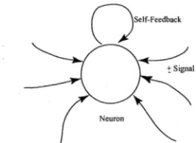
Fig. 2 A neuron with self-feedback
日の色で塗りつぶすこととする.
3. 自己フィードバックを持つニューラル ネットワークに よる四色問題の解法
本節では, 本論文で提案する自己フィード、パックを 持つニューラルネットワークによる四色問題の解法仁 その動作原理を説明する.
3.1 自 己 フ ィ ー ド パ ッ ク を 考慮したニューラ ルネ ッ トワーク
本論文では, McCulloch と Pitts のニューロンモデ ルを用いるうえに, 図 2のように, ニューロンは自己 フィードパックを持ち, ニューロンの制約条件ごとに 図 3に示すようなネットワークを構成すると考えられ る. 図 3のネットワークの各ニューロンは自己フィー ドパックを持ち, ニューロンの出力状態が関係ある制
約条件で構成されるネットワークに結合している. ま た, 各ニューロンの処理を逐次的に行う. ここで, 逐 次的とは, 各ニューロンの処理をした後, 直ちに出力 状態を更新し, それを順番に行うことを意味する.
Fig. 3 Neural network with self-feedback
なお, 提案するニューラルネットワークで、は,ニュー ロンの出力状態は, Takefuji らと同様に McCulloch
Pittsニューロンを用いて, ニューロンが発火するかど うかをそのニューロンの出力状態で判断する.各ニュー ロンの出力は "0"とヲヨ "の二値であり "0"の場合で発
火しないとし "1 "の場合で発火とする. しかし, 本 論文で扱うニューロンは, Takefujiらが使用している ニューロンとは異なり, 内部状態の履歴は持たないも のとし, 変わりに図 2に示すように自己フィードパッ クを持っている. あるニューロンの出力状態がエネノレ ギ一関数を増加させる要因になっていればう出力状態 を反転させる方向に持っていく信号をニューロンに与 える.あるニューロンの出力状態がエネルギ一関数を