Urban Reproduction and Fertility: Kyoto in Late Tokugawa Japan
著者 Hamano Kiyoshi, Mary Louise Nagata journal or
publication title
Kansai University review of economics
volume 16
page range 3‑30
year 2014‑03
URL http://hdl.handle.net/10112/00017198
Urban Reproduction and Fertility:
Kyoto in Late Tokugawa Japan^
Kiyoshi Hamano*
Mary Louise Nagata**
Having collected all of the extant population surveys of Kyoto that included age information, we try to analyze fertility using all data where there were two consecutive listings. The total marital fertility rate was at the low level of 4.03, suggesting that main taining the urban population with fertility alone may have been difficult. This confirms the fertility side of the urban graveyard theory.
Keywords: historical demography, total fertility rate, child-woman ratios, urban grave yard theory
1. Introduction
This investigation of urban fertility in early modern Japan analyzes the popula tion surveys of Kyoto neighborhoods compiled 1842-1869, or the final years of the Tokugawa regime (1600-1868). During the final years of the Tokugawa regime, Kyoto became the focal point for the political conflict of the Meiji Restoration as the official capital and home of the imperial court. Although the main action of the political conflict took place 1860-68, it was preceded by several decades of economic and political instability Patterns of mortality and migration reflect these periods of crisis with increasing levels of mortality and migration from the late 1850s. The political disorder also produced increasing numbers of people who went missing or who
* Professor of Economic History at Faculty of Economics, Kansai University, 3-3-35 Yamatecho, Suita-shi, Osaka 564-8680 Japan. E-mail address: [email protected]
Associate Professor of Asian History, Francis Marion University. 4822 E. Palmetto, Florence, SC USA 29506.
Email address: [email protected]
t Paper presented at the 9th European Social Science History Conference, April 2012, Glasgow, Scotland, UK.
We also gratefully acknowledge the financial support from the JSPS (Grant-in-Aid for Scientific Research
(C) 23530425)
dropped off the record entirely as local authorities found keeping accurate information difficult during the crisis. Analysis of mortality and migration focuses on departures from the data. In this study we address the other side of the demographic story
with fertility.
This study addresses several questions. One is whether and how the fertility level changed over time, especially in response to the decade of political crisis. There was a major famine in Japan in the 1830s followed by an extended economic crisis that particularly affected the Kyoto silk textile industry as a consequence of reforms enacted to address the crisis. Our data begins in the 1840s as the Kyoto economy began recovery from these economic shocks. The 1850s introduced new trouble as the opening of Japan to international trade brought new competition for raw silk to the Japanese economy as well as new opportunities. The 1860s was a new period of political and economic crisis with battles fought in the city streets and a fire burning down two thirds of the city followed by a period of martial law culminating in the downfall of the Tokugawa regime. We find that the total marital fertility rate for Kyoto during these three decades was highest in the 1840s, lowest in the 1850s with a recovery at a median level at the 1860s.
Another question is how the fertility rates for Kyoto compare to village rates in various parts of Japan in relation to the urban graveyard theory. There has been considerable research on the demography of rural villages in various parts of Japan, but much less on that of rural towns and very little on the big cities. The general pattern from the rural data has been low fertility in the northeast, higher fertility in southwestern Japan and highest in the central Japan. However, there has been no research on urban fertility in each of these regions. What little research there has been on urban fertility has focused on rural towns because the larger cities mostly do not have the necessary data. In 2004 we used the data of six neighborhoods for a first analysis of urban fertility, but this data was too limited to credibly analyze differential fertility. This investigation uses the population surveys of twenty-eight neighborhoods, or all of the available extant surveys that provide the best data for analysis of urban mortality in a big city in central Japan. We find that the Kyoto fertility rate was higher than the northeastern village rate, although lower than the village rates for both central and southwestern Japan (Tomobe 1991). These findings seem to confirm the fertility part of the urban graveyard theory, but also that regional differences in fertility rates also mattered.
Finally, we address questions of differential fertility. We find that households with
higher social economic status had higher fertility rates than those with markers of
lower social economic status. These markers included owning vs. renting the resi-
the city. Related to these, we also find that stem family households had higher fertility rates than nuclear households, even though ultimately only one child remained home to succeed to headship of the household.
The next section will explain the historical context of this study followed by an introduction of the data. The following sections will use child-woman ratios and calculation of total and marital fertility rates to investigate differential fertility by socio-economic status, district within the city and decade in relation to the historical context. We also compare the Kyoto fertility rates with those of rural villages in northeast, central and southwest Japan as well as with other urban calculations as available to address the questions of the urban graveyard theory and urban fertility.
2. The Historical Context
Kyoto was the political capital of Japan at the beginning of the Tokugawa period (1600-1868). When Tokugawa leyasu established his government in Edo, Kyoto continued to be the political center for western Japan and a potential focal point for rebellion because the emperor and the old court nobility continued to live there. For this reason, the Tokugawa regime established two offices, the Kyoto deputy {Kyoto shoshidai) and the castellan of Nijo castle {Nijd joban) to represent the shogun's government in western Japan and keep watch over the imperial court. Two city magistrates, the higashi bugyd in the east and the nishi bugyo in the west, were entrusted with the administrative control of the city's other political and legal affairs with a third magistrate, the kura bugyo, in charge of the treasury and financial affairs (Kamada 2000: 343, 353). The details of city administration, however, were controlled by Kyoto neighborhoods. Kyoto neighborhoods had already established an autonomous identity and administration before the mid sixteenth century when Japan's process of reunification began, resulting in the Pax Tokugawa under the Tokugawa regime. The unifiers and the new regime respected this autonomy. Each autonomous neighborhood had its own administrative officials and laws called machi bure or shikimoku although the neighborhoods varied in when they compiled their own laws and how they chose their officials (Kyoto City Library for Historical Documents 1999).
Kyoto neighborhoods were each about one city block in size with all of the resi
dents that lived on either side of the street in that block included in the neighborhood
listings. The administration consisted of an "elder" called the cho toshiyori and three
representatives called gonin gumi. The representatives were technically the heads of
6
five-household responsibility groups from the system of shared responsibility the Tokugawa regime adapted from Ming dynasty China. Kyoto neighborhoods, however, often had forty or more households. The population surveys of Seido neighborhood, for example, record twenty-three official residences and around thirty households per year while Sujiihashi neighborhood surveys record fifty-two official residences and more than seventy households per year. Nevertheless, both neighborhoods had three officials called gonin gumi. Obviously, the gonin gumi represented many more than five households each, even in a small neighborhood like Seido. Although there were differences by neighborhood as to how these officials were chosen for office, the posi tions were often rotated among male heads of household in the neighborhood. The rotation could include all male heads of household or be limited to households that owned their residences or various other criteria determined by the neighborhood.
These officials compiled the annual population surveys and other various surveys and registers required by the state. In the process, they also kept track of births, deaths, marriages, divorces, adoptions, leases of land or housing, wills, debts and other contracts, the travels by heads of neighborhood households, and various moves into and out of the neighborhood. Upon compiling the records, a representative of each household also verified the accuracy of the information with his or her official seal. According to the laws of many neighborhoods, these officials also mediated civil disputes of various kinds and were available to consult for advice (Kyoto City Library for Historical Documents 1999) The data for this investigation of fertility is the population surveys compiled by these neighborhoods 1843-1869. The neighborhoods began compiling these and other registers long before 1843, but most neighborhoods did not record the ages of individual residents before that year^^.
The neighborhoods were grouped with fourteen or so neighborhoods to a group and the elders {cho toshiyori) of these neighborhoods met regularly, exchanging information and sending around any news and new edicts, decisions or requirements of the Tokugawa magistrates and the state. These were recorded in neighborhood journals kept by the elders in a neighborhood office for all to read^^. The neighborhood groups were further grouped in the upper, central and lower capital wards and the eastern hills ward across the Kamo River. An alternative grouping used by the city magistrates in the emergency assistance system divided neighborhoods into "old" and
"new" groups plus some located within temple precincts (Kobayashi 2006: 5). The neighborhoods functioned as autonomous units within the larger administration of the
1) The laws of Takoyakushi neighborhood are explicit about these duties.
2) One neighborhood, Shimizu, recorded age from 1842 and we include that listing in our data sample.
3) Takoyakushi cho, Yashiro Jinbei yaku chu. "Nikki", Takoyakushi neighborhood journal, 1/1/1841-3/2/1842,
Takoyakushi cho collection D2, Kyoto City Library of Historical Documents.
and the political and legal control of the state.
The first year of the data coincides with reforms designed to address economic crisis caused by the Tempo famine of 1836-7. The Tempo famine actually began in 1833 when unusually cold and wet summers produced very poor or no harvests in northeastern Japan. Southwestern Japan was not affected by this problem and harvests were fine, but domains in these areas could be called on to provide emer gency assistance. As the famine continued in the northeast, however, other domains also took action to stockpile their rice in fear that they too would fall short. This meant that the rice reaching the urban consumer markets, such as in Kyoto, was in short supply. The city magistrates could take action against merchants who stock piled their rice looking to make profit on higher prices, but could do nothing about domains that produced rice. Moreover, much of the rice imported to the Kyoto market came by way of the Osaka city markets. When the Osaka magistrates took action to protect the rice available to the people of Osaka, the Kyoto market received less rice. This situation made Kyoto particularly vulnerable to rice shortages and increases in the rice price (Kobayashi 2006: 3-5, 10-13).
Farmers in regions hit by famine typically migrated to or sent family members to the cities in search of work and extra income. Thus there was an influx of cheap labor just as grain prices were rising resulting in wage reductions in the city. At the same time, rising food prices meant that people conserved on other expenses.
Contemporary observers noted that people delayed rebuilding aging houses reducing the employment opportunities for day laborers in the construction industry, so the city magistrates called for more construction to be carried out (Kobayashi 2006: 3 -4). The market for silk brocades and other products of the Nishijin silk textile industry in Kyoto also dried up putting many laborers and artisans that depended on that industry out of work (Hamano 2003).
After the Tempo famine and economic crisis in 1836-7, the Grand Councilor
(tairo) Mizuno Tadakuni enacted a number of reforms to address the economic prob
lems. Two reforms had negative effect for Kyoto and particularly the Nishijin silk
textile industry. The first was a number of edicts that dissolved trade and business
associations or any organization that looked like a guild or a cartel on the assump
tion that these associations were keeping prices high. However, these associations
functioned to regulate the market, manage credit, manage distribution and enforce
contracts. Moreover, many of these associations had been formed by order of the
state in the eighteenth century with the purpose to control prices and keep them
down. The effect of the edicts dissolving and prohibiting these associations was an
upset of the distribution system, lack of credit in a market that operated primarily on credit, and price inflation (Ishii 1991: 78-85, Miyamoto 1938: 330, 337-343). In addition to the negative effect upon the market and the resulting price inflation, the trade associations also had insurance functions that provided assistance to members.
When they were dissolved, this safety net for businesses in times of economic trouble disappeared. This was particularly a problem for the Nishijin textile industry because another part of the Tempo reforms restricted production and sale of luxury items such as silks and introduced new sumptuary laws. So the Nishijin silk textile industry took a direct hit with these reforms, which also removed one of the safety nets for businesses in the industry. Parts of these reforms were rescinded in 1843, the year that our data series begins (Yagi 1982, Hamano 2003: 211).
The immediate cause of crisis in 1853, however, was a fourteen percent jump in the price of rice due to another poor harvest. In autumn of 1852 the price was already higher than usual at 101.8 monme (381.8 grams) of silver and it jumped to 116 monme (435 grams) of silver in 1853 (Mitsui Bunko 1989: 106)'^^. 1853 was also the year that the American Commodore Matthew Perry forced Japan to open wider to international trade. By 1857 Japan had treaties with five Western nations and had opened several new treaty ports. The opening of the treaty ports contributed to the economic growth of some parts of Japan, especially regions in the northeast that produced raw silk. However, raw silk that was exported abroad was also raw silk that did not reach the Kyoto market. This caused the price of raw silk to rise in Japan bringing a supply crisis to the silk textile industry that now found itself in competition to buy raw silk. At the same time, brokers who dealt in raw silk took advantage of the rising prices and stockpiled the silk. In 1863 one such broker's warehouse was attacked revealing a stock of 500,000 ryo of raw silk at a time when finding raw silk for sale in the market was difficult (Mitsui Bunko 1989: 106).
In 1854 the Tokugawa regime under Grand Councilor {tairo) li Naosuke added another level of administration to the city by establishing the Kyoto warden {Kyoto shugo) to take charge of the city and its defense. This new post was a reaction to the foreign threat brought by the forced opening of Japan and foreign pressure to sign treaties and trade agreements with five European nations. The imperial court in Kyoto gained renewed significance and political voice as forty daimyo also gath ered in Kyoto under the Kyoto warden and Kyoto deputy ready to defend the city and the court from the foreign threat (Kyoto City 1970: 596-597, Kamada 2000: 354).
After the post of Kyoto warden was established in 1854, a fire broke out burning
4) One monme is 3.75 grams.
some five thousand residences in the northwestern part of the city (Kyoto City 1979:
609, Akiyama 1980: 334). There were also two major earthquakes in 1854, the Ansei Tdkai earthquake along the coast between Nagoya and Edo and the Ansei Nankai earthquake affecting the coastal region directly south of Kyoto both estimated 8.4 on the Richter scale and with accompanying tsunami. Neither of these earthquakes were close enough to be felt in Kyoto, although the fire may have been related to it, but they likely sent refugees to Kyoto as well as Osaka and may have had other negative effects upon the urban economy.
In 1862 the Tokugawa regime and the imperial court acted on a plan to unify court and shogunate called kobu gattai and the shogun Tokugawa lenari moved to Kyoto. Shimazu domain sent military forces to Kyoto demanding the return of political authority to the imperial court and in 1863 a shogunal army of 1600 men also marched on Kyoto in response, but were persuaded to leave. lenari also returned to Edo while in Kyoto the Satsuma-Aizu domain alliance that supported the unifica tion plan forced the group led by Choshu domain that demanded return to imperial rule out of the city. This process also included political violence with assassinations and fighting in some streets. Commanders of the shogunal forces used the offices of neighborhood administrations for their military command headquarters potentially disrupting the record keeping process.
Young warriors that were Tokugawa loyalists also formed a vigilante group called the Roshi gumi and continued opposition to the supporters of the demand to return to imperial rule with assassinations and random attacks. In 1864, military forces from Choshu domain invaded Kyoto and fought against Tokugawa loyalists at the west gate of the imperial palace invading the palace grounds at the Nakadachiuri street gate. The Choshu domain mansion was set afire and a number of private homes near Nakadachiuri were attacked and also set afire. Fire spread burning many buildings down from Ichijo street in the north to Nanajo street in the south, or approximately two thirds of the city including most of the commercial center and much of the southern periphery. Of course 1864 was not the end of the political conflict, but there were no more major incidents of political violence in the streets of Kyoto, although the city was under the domination of vigilante loyalists called the Shinsengumi charged with maintaining order from 1864 until the fall of the Tokugawa regime in 1868.
In addition to the political crises of the 1860s, the price of rice also reveals an
economic crisis that continued after the battle and fire of 1864. The price of rice
that had already jumped rather high to 154.5 monme in 1858 and 221.1 monme in
1860, more than doubled to nearly 500 monme in 1865 and again to nearly 1200
10
monme in 1866. This combination of political and economic crises suggests that the mortality rate in Kyoto may have been higher than "normal" for the city, at least during the 1860s and this could have produced a rebound reaction in fertility The next section introduces the data and methodology for this analysis.
3. Data and methodology
The data for this study is the religious and population surveys called Shumon Ninbetsu Aratame Cho of twenty-eight neighborhoods in Kyoto: 11 neighborhoods in or near the commercial center, 7 neighborhoods in the Nishijin silk district, and 10 neighborhoods on the outer edges of the city in each direction excluding Nishijin in the northwest (See the map for the geography of the three districts). The surveys provide listings of neighborhood residents submitted in the ninth month of the lunar calendar by each neighborhood community. The surveys list each resident of the neighborhood by religious sect (all Buddhist), and household of residence by name and relation to the head of household. From 1843 the listings also record the age and birth province of each individual and made greater effort to keep track of move ment into or out of the community through notations on slips of paper pasted on the surveys. In addition, the ninth month listing each year was followed by an update listing of newcomers to the neighborhood in the second lunar month of the following year. These changes were probably related to the Tempo reforms. These annual listings continued until 1868, the year the Tokugawa regime fell, although some neighborhoods also compiled a final listing in 1869. Since age and birth province are important information for identifying and linking individuals from one listing to the next and age is essential for any demographic analysis, this study uses only the list ings compiled 1843-1869. We use consecutive listings and, where possible, the second
month update listings to also calculate infant mortality.
Japanese institutions did not keep records of births or marriages on a systematic basis except for the information in the population surveys^^ They were more inter ested in who was there, including children who survived, rather than those who were absent or dead. In analysis of marriage patterns, we used the presence of a co-resi dent child or co-resident spouse as evidence of marital experience (Nagata and Hamano 2009). For this analysis, we limit our analysis of "marital fertility" to women who have co-resident spouses acknowledging that these women are only a subset of married women and that we have no way to measure categories of widowed,
5) For the legal use of the population surveys as evidence of marriage, see Nagata (2003a).
©Sujiihashi
©Kankiji ©Shimoyanagi South
©Hanakuruma ©Shibayakushi
@Ubagaenoki|H|isJiijin
©Jozenji
OMatsuue
ONishinokyo Kamino
* •Saihoji
} ; ©Takoyakushi f
•Sorin
Cbmmetci^l Center
^ i
^ * t
•Kawatana©Tachiuri Nakanocho
•Minami Shijo
; #Sann6^_
^Taishiyama | .
©Yoshimizu
ii OKanaya
r/ Olshigaki West
I ODaikoku
I ODaibutsu Shomen I
OKami Ninomiyans^
OKanegae OShimizu
Sanjo St.
Shijo St.
Map of Kyoto and 28 neighborhoods providing data
# Commercial Center © Nishijin OEdge
divorced or married-living-separate-from-spouse because the surveys do not record non-resident kin. Since we do not really have records of births, we begin our analyses with "own-children" analyses and child-woman ratios for this investigation of fertility patterns.
Children started entering service in large numbers from age 10 and large propor tions of the people in the data set ages 10-25 were servants (see figure 1). Those
children who were not sent into service or apprenticeship for their education and
training were sometimes sent to boarding schools or established in separate house
holds as branch shops of their family's business to begin intensive training. This
12
300 r
800 ^
sib
"" < /Is-:
600 4 JiM
500 . -V,
400
V-' /, "
300 :fV
V''<y
'- - - - t- ^ vo.5s^s-
0 WWWWWWWWWBWWWWWBHWBWWBMi^^ -,
1 3 5 7 9 11 13 15 17 19 21 23 25 27 29 31 33 35 37 39 41 43 45 47 49 51 53 55 57 59 61 63 65 67 69 71 73 75 77 79 81 83 85 87 89 91 93 Age
Figure 1 Total Observations by Age and Relation to Head
process occurred with several children in the Takoyakushi data from around age 8.
These complications mean that using own children ages 1-15 (0-14 in Western reck oning) to estimate fertility is highly unreliable, so we limit our examination to chil dren ages 1-5 (0-4 in Western reckoning).
Adoption adds another complication to the analysis. Adoption to recruit an heir, for alliances between families and as ways to find caregivers for foundlings and other problem children was a common practice in Kyoto at this time. However, the surveys largely do not record adoptive relationships. Analysis of adoption, however, has shown that most adoption took place with older children and adults (Nagata 2003b). Since adoptive "fictive" kin relations are often impossible to identify, we assume that chil dren ages 1-5 who are identified as "son" or "daughter" of the head of household are the natural children of the woman identified as "wife" even though the "wife" might be the second wife after the natural mother died or was divorced, or the children may have been adopted.
These listings provide 32,062 person years for analysis from a total of 175 flat file listings when not examining change from one year to the next. Using these list ings for longitudinal analysis, however, reduces the data considerably. Seven of the eleven neighborhoods in the city commercial center provide listings for two or more consecutive years for analysis of change from one year to the next, only two with substantial time series. The population series for these neighborhoods shown in figure 2 show a rather flat trend of stable population during most of the data period, but the year 1864 was clearly a problem for the one neighborhood, Nishido, providing
continuous data for the 1860s.
•— Yoshimizu Nakanomachi Sorin
>»»«»Nishido
^Taishiyama
—Takoyakushi
—Toro
• Minamishijo
1843 1848 1853 1858 1863 1869
Figure 2 Neighborhoods in the Commercial Center
Three of the seven neighborhoods in Nishijin provide consecutive year data, two with substantial time series. Plotting the observed population of each neighborhood per year reveals that Nishijin, shown in figure 3, followed a different population trend from the city center. These neighborhoods show signs of growth 1843-55 consistent with rebound in the silk textile industry after the Tempo austerity reforms were rolled back. This is followed by decline consistent with the effect of inflation in the price of raw silk related to the opening of the ports to international trade and the higher prices paid by foreign merchants. Price inflation also affected food prices and several neighborhoods have records of hardship distributions in 1861. After 1861, however, the Nishijin population trend shows growth. Nishijin was north of the great fire of 1864 and likely received some refugees from the fire and from the political conflict before and after the fire. As yet, however, no individuals from any neighbor hood have been identified in any other neighborhood in the data. This is probably because only twenty-eight neighborhoods have data available for analysis out of a total of 1600 neighborhoods comprising the city at that time. The data from one neighborhood, Kankiji, shows the full trend of change over time, but the other shorter neighborhood series from Hanakuruma and Sujiihashi also reflect these trends.
The other peripheral neighborhoods are even more problematic for examining
change from one year to the next. Only four of the ten neighborhoods from the city
periphery provide two or more consecutive years of data and the time series are
quite fragmentary. Limiting the data to samples with two or more consecutive years
thus reduces the sample to 18,819 person year observations from years where there
is a listing for the following year in fourteen neighborhoods. Despite the neighborhood
14
distribution, however, the person years divide fairly equally between 8,300py from the city center and 8,322py from Nishijin with a much smaller sample of 2,197py from the other peripheral neighborhoods. Figures 2 and 3 reveal that the combined samples from the city center and from Nishijin provide a continuous or near contin uous time series through the data period. The samples from the periphery, however, do not as shown in figure 4. On the other hand, the peripheral neighborhoods providing this data include one from the western, two from the southern and one from the eastern edges of the city. None of these neighborhoods was affected by the
— Hanakuruma
«~~»Kankiji
— Sujikaibashi
Figure 3 Neighborhoods in the Nishijin silk textile district
—Kanaya
—Kanegae
—Shimizu
— Kamininomiya
• - - Nishinokyo kaminocho
— Ishigakicho Nishigawa
Figure 4 Neighborhoods in the periphery, but not in Nishijin
fire in 1864, but the western neighborhood, Nishinokyo Kaminocho, was involved in the conflict and the population rebounded after the conflict as shown in the rising population trend from 1865.
4. Child-Women Ratios
Most of the data series from the twenty-eight neighborhoods providing data for our sample are spotty with many gaps and many neighborhoods providing only one listing, several years without consecutive listings, or limited consecutive listings. In addition, mobility was high with an average population turnover per neighborhood of twenty percent per year, so even in data series that contribute multiple consecutive listings few individuals can be observed over long periods of time. A total of 1,691 children appear in the data for the first time at recorded ages 1-5 and they are observed in the data a total of 2,874 times meaning each child contributed an average of 1.7 observations. At the same time, 6,512 females appear in the data of which 3,389 appear for the first time at ages 16-45 and the total number of person year observations for women ages 16-45 is 7,786. We use the women ages 16-45 instead of women ages 16-50 because only two children were born to women ages 46-50 so the numbers are too small to be meaningful. Since many women observed during this age period may have entered the data before the age of sixteen, 3,687 is an underestimate of the number of women observed at ages 16-45. So the average number of observations per woman is less than 2.3, which is not very different from the average for the children. For these reasons, all analyses for this study will be in person years and we begin the analysis with child-woman ratios shown in table 1.
The child-woman ratio (CWR) for the entire data sample is 0.369.
Life-cycle service complicates the analysis of fertility for Kyoto. Figure 1 reveals that the number of people observed in the data at ages 11-25 is greatly inflated due to life-cycle service and figure 5 confirms that this is true for women at ages 16-25.
Many of the women at these ages were servants and servants are not at risk of
being recorded with children in the data. This does not mean that servants did not
bear children, but those children would be sent home to the mother's family or the
father's family and very few children could not be linked to legitimate mothers in
the data. Therefore, servants were not at risk for fertility. Therefore, where servants
were common CWR was likely to be low as can be seen in the comparison of house
holds with co-resident servants having a CWR of 0.256 and households without
servants having a CWR of -.427. When the servants are removed from the calcula
tion, the households employing servants had a CWR of 0.500. In other words, the
16
family that employed servants had a higher fertility rate than the family without servants on average, but including servants in the calculation diluted the effect.
The table shows comparisons of CWR for various categories of women and households. We presume that households that owned their residences were generally
Table 1 Child-Women Ratio: Kyoto 28 neighborhoods
CWR child
population
women age 16
women age 16 -45 excluding -45
servants
CWR excluding
servants
Owner 898 3024 2074 0.297 0.433
Renter 1975 4762 4422 0.415 0.447
With servant 677 2645 1355 0.256 0.500
Without servant 2196 5141 5141 0.427 0.427
1842-1849 990 2907 1940 0.341 0.510
1850-1859 943 2325 2280 0.406 0.414
1860-1869 940 2554 2276 0.368 0.413
Center 1139 3313 2409 0.344 0.473
Nishijin 1201 3179 2833 0.378 0.424
Edge 533 1294 1254 0.412 0.425
Nuclear 1869 4953 4350 0.377 0.430
Stem 784 1922 1436 0.408 0.546
Extended 166 542 434 0.306 0.382
Total 2874 7786 6496 0.369 0.442
* Renter includes a few borders.
S'iliii;
oarent
1 3 5 7 9 11 13 15 17 19 21 23 25 27 29 31 33 35 37 39 41 43 45 47 49 51 53 55 57 59 61 63 65 67 69 71 73 75 77 79 81 83 85 87 89 91 93
Figure 5 Female Observations by Age and Relation to Head
more affluent than those who rented. Similarly, households with co-resident servants or employees were generally more affluent than those without any servants and many of those with servants were also successful businesses. We also compared the various decades of the data in consideration of the historical context and the earliest period when the economy was most stable had the highest CWR. In addition, house holds in the commercial center had higher ratios than others and stem family house holds also had more children per woman. Other studies have shown that households in the commercial center were more likely to be larger, successful family businesses and the family businesses that employed many servants were more likely to be observed as stem family households for reasons of apprenticeship and headship succession, so these results fit the picture of successful family businesses also having more children. On the other hand, once servants were removed from the calculation, there was no substantial difference between owners and renters.
5. Age-specific fertility rates
In this section we address age-specific fertility and differential fertility to compare fertility under various conditions. Calculation of age-specific fertility from the population surveys requires some adjustments. The population surveys were compiled in the eighth month of the lunar calendar and submitted to the political authorities in the ninth month, so a child listed as age one in year x was born some time between the first and seventh months of the year. As noted above, the age recorded in the listings represents the calendar year of life and not time elapsed since birth. A child listed for the first time as age two as a child of parents listed in the household the previous year was born between the eighth and the twelfth months of the previous year (Hamano 2007: 65^66). Therefore children born in year X include children listed that year as age one and children recorded for the first time the following year as age two. Of course, children born after the listings were compiled do not appear the year they were born, but appear the following year if they survived to be counted. In some neighborhoods, children born after the listing for one year was compiled may be listed in the newcomer update listing added in the second month of the following year, but this was rare. The analyses in this section are entirely comparisons of differential fertility from within the data sample.
Since all of the data is subject to the same limitations, we do not use the second month listings to maintain consistency within the data in comparison®'. Of course we
6) In our previous analysis we found 15 children listed at age one in the second month update from two
neighborhood listings of which 13 appeared in the ninth month listings of the same year and calculated
18
have no information about children who were born and died in between listings so our calculations of fertility and infant mortality may underestimate the levels.
Since the children born in any year are recorded in the listings of two consecu tive years, we limit the data sample to only those neighborhood series that provide at least two consecutive listings to calculate infant mortality. As a result, the new sample is limited to sixteen neighborhoods and 105 listings. Table 2 and figure 6 show the age-specific fertility and marital fertility rates. These figures are clearly affected by the presence of many female servants in the data as noted in the previous section above and they serve to depress the age specific fertility rates. For this reason, we also include the marital fertility rate. For this analysis we define married as women having a co-resident spouse. The listings provide no information of whether a woman was divorced or widowed or living separate from her spouse, so this is the only information available to determine the marital status of a woman besides the presence or absence of children. Thus, the numbers of married women are also necessarily underestimated. At the same time, few women can be identified as married before the age of 23, so the marital fertility rate for women ages 16-20 will be overestimated simply because there are so few of them. For this reason, we calculate the rates for women 16-50 and also 21-50.
The rates in table 2 and the following tables in this section refiect calculations using the entire data set from twenty-eight neighborhood samples, thus the total fertility rate (TFR) of 2.19 and the marital fertility rate (TMFR) of 3.09 are really the general rates that have not been adjusted for infant mortality. We will consider the adjustments to these rates in the next section. At this time we compare these
Table 2 Age-Specific Birth Rates: Kyoto 28 neighborhoods (A) All Births
Fpmiiip Married Age-Specific Age-Specific Births py married women Fertility Marital
women PY Rate Fertility Rate
1 - 0.9 - 0.8 ^ 0.7 » 0.6 -
16-20 16 888 12 80 0.090 0.750 0.5 -
21-25 70 902 66 368 0.388 0.897 0.4 *
26-30 109 830 108 593 0.657 0.911 0.3 ^
31-35 82 723 79 590 0.567 0.669 0.2 -
36-40 49 721 44 557 0.340 0.395 0.1 -
41-45 15 627 15 441 0.120 0.170 0 *
46-50 3 500 2 306 0.030 0.033
16-50 21-50
344 328
5191 4303
326 314
2935 2855
2.191 2.101
3.825 3.075
16- 21- 26- 31- 36- 41- 46- 20 25 30 35 40 45 50
—❖»«» Age-Specific Fertility Rate -♦-Age-Specific Marital Fertility Rate
Figure 6
an IMR of 240. See Nagata and Hamano (2004).
raw rates with the child-woman ratios in the various categories of the previous
section.
Table 3 and Figure 7-8 compare the fertility rates of owners and renters. The TFR for renters is higher than for owners, but this may reflect the fact that owners were also more likely to employ co-resident servants. The relation reverses for TMFR which does not include servants because no servants are observed as married. In the child-woman ratios, however, although removing servants from the calculation greatly increased the CWR for owners, the rates for renters remained higher than for owners in both cases (see table 1).
Table 3 Fertiltiy of owners and renters (A) Owners
Female ^11 Births
Age Female PY
Births
(Married) PY(Married) Age-Specific Fertility Rate
Age-Specific Marital Fertility
Rate
16-20 6 516 5 40 0.058139535 0.625
21-25 19 458 18 126 0.207423581 0.714285714
26-30 44 325 43 193 0.676923077 1.113989637
31-35 26 218 25 164 0.596330275 0.762195122
36-40 11 197 10 130 0.279187817 0.384615385
41-45 9 206 9 133 0.218446602 0.338345865
46-50 1 190 1 126 0.026315789 0.03968254
16-50 116 2110 111 912 2.062766676 3.978114263
21-50 110 1594 106 872 2.004627142 3.353114263
(B) Renters Female
ages
Female PY
Births to married
women
Married women PY
Age-Specific Fertility Rate
Age-Specific Marital Fertility
Rate
16-20 10 372 7 40 0.134408602 0.875
21-25 51 444 48 242 0.574324324 0.991735537
26-30 65 505 65 400 0.643564356 0.8125
31-35 56 505 54 426 0.554455446 0.633802817
36-40 38 524 34 427 0.36259542 0.398126464
41-45 6 421 6 308 0.071258907 0.097402597
46-50 2 310 1 180 0.032258065 0.027777778
16-50 228 3081 215 2023 2.37286512 3.836345193
21-50 218 2709 208 1983 2.238456518 2.961345193
Age-Specific Marital Fertility Rate Age-Specific Fertility Rate
16-20 21-25 26-30 31-35 36-40 41-45 46-50
— Owner - Renter
Figure 8
16-20 21-25 26-30 31-35 36-40 41-45 46-50
—^Owner Renter
Figure 7 Owners and Renters
20
Table 4 and figure 9-10 compare the fertility rates of households that had co-resident servants and those that had no co-resident servants. Most of the house holds that had co-resident servants were also units of family businesses and the
"servants" included business employees such as clerks, weavers, apprentices and other positions related to the business. This comparison, therefore, is like the previous comparison of more affluent households with less affluent households. Most of the households with co-resident servants owned their residences, but some rented. Most of the households that rented their residence employed no co-resident servants, but some households without servants owned their residence. So, the correspondence is
Table 4 Fertility in households with servants and without servants (A) With Servant
Female
ages Births Female PY
Births to married
women
Married women PY
Age-Specific Fertility Rate
Age-Specific Marital Fertility Rate 16-20
21-25 26-30 31-35 36-40 41-45 46-50
4 12 32 24 6 8 0
558 439 292 188 130 112 105
4 11 32 24 4 8 0
29 80 175 148 85 82 76
0.036 0.137 0.548 0.638 0.231 0.357 0.000
0.690 0.688 0.914 0.811 0.235 0.488 0.000 16-50
21-50
86 82
1824 1266
83 79
675 646
1.947 1.911
3.825 3.136 (B) Without Servant
Female g;
ages Female PY
Births to married
women
Married women PY
Age-Specific Fertility Rate
Age-Specific Marital Fertility Rate 16-20
21-25 26-30 31-35 36-40 41-45 46-50
12 58 77 58 43 7 3
330 463 538 535 591 515 395
8 55 76 55 40 7 2
51 288 418 442 472 359 230
0.182 0.626 0.716 0.542 0.364 0.068 0.038
0.784 0.955 0.909 0.622 0.424 0.097 0.043 16-50
21-50
258 246
3367 3037
243 235
2260 2209
2.536 2.354
3.835 3.051
Age-Specific Fertility Rate Age-Specific Marital Fertility Rate
46-50 21-25 26-30 31-35 36-40 41-45
—O"—With Servant ^ Without Servant
21-25 26-30 31-35 36-40 41-45
—^With Servant Without Servant
Figure 9 Figure 10
not complete, but the trend is there. In this case, the TFR was higher for households without co-resident servants, again reflecting the effect of female servants in the calculation, but the TMFR was nearly the same, whereas the CWR for households without servants was higher than the rate for households with servants until the servants were removed from the calculation when the relation between the rates reversed. Considering the effect life-cycle service had upon the various measures of fertility, the marital fertility rate is more accurate. At the same time, we must remember that the small numbers of women married before the age of 20 also has an effect on the calculation, so the marital fertility rate for women over the age of 20 is the best one to use. This is also reasonable because in other research we have demonstrated that nearly all women married and there is no true illegitimacy rate (Nagata and Hamano 2009).
The Kyoto population surveys identify the birth province of each individual and this is our clearest information on migration. Since this information only identifies the province, we cannot identify all those who immigrated to the city because many may have come to the city from villages in the same province Kyoto was located in.
Therefore, to compare the fertility behavior of Kyoto natives with immigrants we actually compare the behavior of individuals born in Yamashiro province that included Kyoto, or Yamashiro natives, with those born in other provinces. There was very little difference in the two rates, partly because most "immigrants" who remained in the city after completing their service married and the majority married natives. Moreover, not only did non-native women marry native men, but non-native men often married native women (Nagata and Hamano 2009). The two figures accompanying the table 5, figures 11-12, however, reveal that non-native women married later than Yamashiro natives and stopped bearing children sooner. Thus, for their marital fertility rates to have been nearly equal, non-native women had to produce children at a faster pace than native women.
The historical context explained in a previous section above shows that the three
decades of our data each had very different political and economic circumstances
with the 1840s as most stable and the 1860s as least stable with both political conflict
and economic hardship. In other research we have found effects of this context in
mortality rates. Table 6 and figure 13-14 compare the three decades to see if there
was an effect in fertility rates as well. The calculation of mortality for the 1860s
was complicated by the large numbers of people who either dropped off the record
or went missing. Although many children may have been born and died between
registrations, increasing the infant mortality rate in ways we cannot observe, we can
calculate fertility rates based on the families and mothers that remained in the data.
22
Table 5 The fertility of Yamashiro natives and non-natives (A) Yamashiro Native
Female Female PY
ages
Births to married
women
Married women PY
Age-Specific Fertility Rate
Age-Specific Marital Fertilitv Rate
16-20 16 695 12 79 0.759
21-25 65 710 61 345 0.458 0.884
26-30 96 706 95 529 0.680 0.898
31-35 67 629 64 506 0.533 0.632
36-40 43 620 38 473 0.347 0.402
41-45 15 535 15 371 0.140 0.202
46-50 3 427 2 255 0.035 0.039
16-50 305 4322 287 2558 2.192 3.817
21-50 289 3627 275 2479 2.192 3.057
(B) Non-Native Female o-
Births ages
Female PY
Births to married
women
Married women PY
Age-Specific Fertility Rate
Age-Specific
Marital Fertilitv Rate
16-20 0 193 0 1 0.000 0.000
21-25 5 192 5 23 0.130 1.087
26-30 13 124 13 64 0.524 1.016
31-35 15 94 15 84 0.798 0.893
36-40 6 101 6 84 0.297 0.357
41-45 0 92 0 70 0.000 0.000
46-50 0 73 0 51 0.000 0.000
16-50 39 869 39 377 1.749 3.353
21-50 39 676 39 376 1.749 3.353
Age-Specific Fertiiity Rate Age-Specific Marital Fertiiity Rate
21-25 26-30 31-35
—^Yamashiro Native
36-40 41-45 Non-Native
21-25 26-30 31-35
■—O"* Yamashiro Native
36-40 41-45 Non-Native
Figure 11 Figure 12
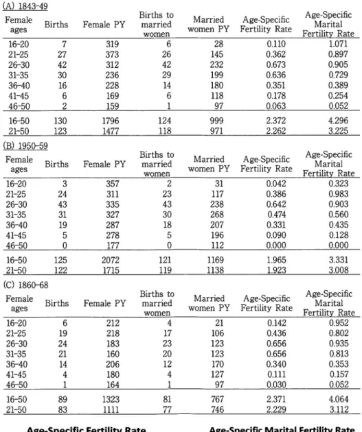
There does not appear to be a large difference in fertility rates between the first and third decades, but the trend seems to suggest that the uncertainty of the 1850s suppressed the fertility rate, while the excess mortality from political conflict in the 1860s may have served to raise fertility again. In this case the fertility trend differs from the child-woman ratios where the 1850s had the higher rate.
The data sample comes from neighborhood collections from across the city and
the different districts, as in many cities, represent different social and economic
characteristics. We have divided the neighborhoods into three groups: the commercial
center, the Nishijin silk textile district, and other neighborhoods located on the outer
Table 6 Fertility and the historical context (A) 1843-49
Female
ages Births Female PY
Births to married
women
Married women PY
Age-Specific Fertility Rate
Age-Specific Marital Fertility Rate 16-20
21-25 26-30 31-35 36-40 41-45 46-50
7 27 42 30 16 6 2
319 373 312 236 228 169 159
6 26 42 29 14 6 1
28 145 232 199 180 118 97
0.110 0.362 0.673 0.636 0.351 0.178 0.063
1.071 0.897 0.905 0.729 0.389 0.254 0.052 16-50
21-50
130 123
1796 1477
124 118
999 971
2.372 2.262
4.296 3.225 (B) 1950-59
Female
ages Female PY
Births to married
women
Married women PY
Age-Specific Fertility Rate
Age-Specific Marital Fertility Rate 16-20
21-25 26-30 31-35 36-40 41-45 46-50
3 24 43 31 19 5 0
357 311 335 327 287 278 177
2 23 43 30 18 5 0
31 117 238 268 207 196 112
0.042 0.386 0.642 0.474 0.331 0.090 0.000
0.323 0.983 0.903 0.560 0.435 0.128 0.000 16-50
21-50
125 122
2072 1715
121 119
1169 1138
1.965 1.923
3.331 3.008 (C) 1860-68
Female
ages Female PY
Births to married
women
Married women PY
Age-Specific Fertility Rate
Age-Specific Marital Fertility Rate 16-20
21-25 26-30 31-35 36-40 41-45 46-50
6 19 24 21 14 4 1
212 218 183 160 206 180 164
4 17 23 20 12 4 1
21 106 123 123 170 127 97
0.142 0.436 0.656 0.656 0.340 0.111 0.030
0.952 0.802 0.935 0.813 0.353 0.157 0.052 16-50
21-50
89 83
1323 nil
81 77
767 746
2.371 2.229
4.064 3.112
0.8 0.7 0.6 0.5 0.4 0.3 0.2 0.1 0
Age-Specific Fertility Rate Age-Specific Marital Fertility Rate
11
^ _