Instructions for use
A uthor(s ) Ohtsuka,T akeshi; T sai,Y en-Hsi R .; GIGA ,Y OS HIK A Z U
C itation Hokkaido University Preprint S eries in Mathematics, 1099: 1-25
Is s ue D ate 2017-1-5
D O I 10.14943/84243
D oc UR L http://hdl.handle.net/2115/69903
T ype bulletin (article)
F ile Information pre1099.pdf
SEVERAL DISLOCATION CENTERS
TAKESHI OHTSUKA, YEN-HSI RICHARD TSAI, AND YOSHIKAZU GIGA
1. Introduction
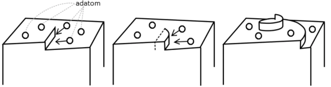
We are interested in modeling and simulation of growth of crystal sur-faces that have discontinuities in height along curves that spiral out from a few centers. The centers correspond physically to the end points of screw dislocation in the crystalline structure. Due to the dislocations, the crystal surface have discontinuities which are generally referred to as steps. Spiral steps evolve by catching atoms on the surface, and the increase in crystal height could be thought of as the spiral steps climbing up the helical surface provided by lattice structure of atoms including screw dislocations. We refer such type of crystal growth as “screw dislocation aided crystal growth”.
Figure 1.1. Illustration of crystal growth with aid of screw dislocation.
Since the spiral dynamics of several screw dislocations involve merging of different spirals, implicit interface methods are attractive options for de-scription of the spiral steps. See [14, 15, 13] for details of the conventional level set methods, [3] for its foundation in mathematical analysis. For spiral curves, see the level set formulation introduced in [10] and [9]. On the other hand, a phase-field approach for evolving spirals are introduced by [5, 6, 7].
The first author is partly supported by the Japan Society for the Promotion of Science through grants No. 26400158(Kiban C).
The second author is partly supported by NSF grant DMS-1318975.
The third author is partly supported by the Japan Society for the Promotion of Science through grants No. 26220702(Kiban S) and No. 16H03948(Kiban B).
In this paper, we study the growth rates of such crystals as described in [1] using the method proposed in [9]. In particular, we give a quantitative definition of the critical distance (of co-rotating screw dislocations) under which the effective growth resembles that of a single spiral. We conclude that the critical distance in [1] is too small compared with our definition. We further give some improved estimates of the growth rate of crystal sur-face by co-rotating spirals. Finally, we present a numerical study on growth rates by a group of screw dislocations. In particular, the influence of dis-tribution screw dislocations in a group of them is considered. Recently, Miura–Kobayashi [7] proposed a phase-filed formulation for spiral crystal growth, and they concluded that their numerical simulations agree with the prediction of Burton et al [1]. One of the aims of this paper is to clarify some discrepancy between the growth rates computed by our method and those reported in [1] and [7]. Moreover, we study on the growth rate by a group including several rotational orientation, which is mentioned in [1] and not treated in [7].
The numerical simulations reported in this paper were computed by an implementation of the algorithm proposed in [9], and it is reviewed in the next section.
2. Preliminaries
In this section we recall the level set method [10, 9] for evolving spiral steps by (2.1) on the crystal surface. The method also includes a way to reconstruct the crystal surface from the solution of the level set equation.
We consider a growing crystal surface that contains spiral steps attached to many screw dislocations. These steps are modelled as curves inR2in this paper, and we will use “curves” or “steps” interchangeably in this paper. According to the theory of Burton et al, [1], spiral steps move with normal velocties given as
(2.1) V =v∞(1−ρcκ),
where κ is the curvature corresponding to the inverse direction of the evo-lution of steps, v∞ and ρc are positive constants describing the velocity
of straight line steps and the critical radius of the two dimensional kernel, respectively.
When a single spiral step with a height, h0 > 0, steadily rotates with angular velocity ω, then the surface grows with the vertical growth rate
R= ωh0 2π .
Burton et al. [1] calculated ω by approximating the form of the spiral step with an Archimedean spiral, and then they obtained thatω=v∞/(2ρc).
were discussed. However, it was pointed out that the estimate on the growth rate for such setups was not accurate.
2.1. Description of spirals. Let Ω be a bounded region in R2, and
a1, a2, . . . , aN ∈Ω be the centers of the spirals. Define
W = Ω\
N
∪
j=1
¯
Br(aj),
whereBr(aj) is a disc with radiusr centering ataj. We assume that ¯Br(aj)
do not intersect.
In our method, spirals are implicitly defined by two functions,u andθas follows:
Γt:={x∈W|u(t, x)−θ(x) = 2πn, for some integer n}.
(2.2)
Correspondingly, we define the orientation of a spiral by n=−|∇∇(u(u−−θ)θ)|.
θ(x) is a pre-determined function of the form
(2.3) θ(x) =
N
∑
j=1
mjarg(x−aj).
This function reflects the sheet structure of the lattice of atoms with screw dislocations, and it was first proposed by [6] to model spiral curves. The constantsmj define the strengths of the spiral centers: each strength is the difference between the stength, m+j , of counter-clockwise rotating spirals (that are attached to aj) and m−j for the clock-wise rotating ones. See [9, Definition 3,5] for details on mj.
The functionu(x, t) is called an auxiliary function to be approximated by solving a partial differential equation inW with suitable initial and bound-ary conditions:
(2.4) ut−v∞|∇(u−θ)| {
ρcdiv ∇(u−θ)
|∇(u−θ)|+ 1 }
= 0 in (0, T)×W,
with an initial value conditionu(0, x) =u0(x) forx∈W for a continuous
functionu0 on W satisfying
(2.5) Γ0={x∈W|u0(x)−θ(x) = 2πnfor an integer n}.
We impose the right angle condition between Γt and the boundary of W,
which is denoted by ∂W. This condition is given as
(2.6) ⟨⃗ν,∇(u−θ)⟩= 0 in (0, T)×∂W,
A few remarks are in order. First, the discontinuity of θ does not cause any problem in (2.4) since ∇θcan be defined uniquely. In fact, ∇θ is well-defined onW as
∇θ=
N
∑
j=1 mj
|x−aj|2(−x2+aj,2, x1−aj,1)
for x = (x1, x2) and aj = (aj,1, aj,2) by taking a branch of θ so that it is
smooth aroundx.
Second, notice thatu0 satisfying (2.5) is not unique even if u0 is consid-ered in the space of continuous functions. However, the uniqueness of Γt
for a given Γ0 is established in [4] provided that u0 is continuous and the
orientation of Γ0 given by u0 is same. In order words, Γt depends only on
Γ0 and its orientation, and is independent of the choice of the functions that
embed it.
2.2. Growth rate of the surface. With given θ and u, Γt is defined,
and the height function the growing crystal surface is defined as
h= h0
2πθΓt(x),
where θΓt is a branch of θ that has 2π-jump discontinuity only on Γt; see
[9]. We define the mean growth height in the time interval [t0, t] as
H(t;t0) =
1
|W|
∫
W
(h(t, x)−h(t0, x))dx,
where |W| is the area of W. Here and hereafter we shall use a notation
H(t) :=H(t; 0) unless it is necessary to clarify the initial time t0.
The growth rate of the crystal surface is then given formally by
R(t) =H′(t;t0) = 1
|W|
∫
W
ht(t, x)dx.
However, H(t) may not be differentiable somewhere and may have oscilla-tions with small amplitudes due to the domain shape. Therefore, in this paper, we computed an “effective” growth rate of the crystal by a linear approximation that best fit, in the sense of least square, the numerically computed values of H(tj) for tj in a chosen time interval. More precisely, we calculateR△ minimizing
(2.7) min
R△ K
∑
j=0
|H(t0+j∆t, t0)−R△(j∆t−t0)|2
with ∆t= (t1−t0)/K for someK ∈Non a time interval [t0, t1]. Then, the
3. New estimates of the growth rates and numerical results
In this section, we discuss old and new estimates of crystal growth rates under different configurations of screw dislocations. Our discussion is ac-companied by the corresponding numerical simulations which serve both as motivation and verification of the reported new results.
3.1. Discretization and numerical parameters. We discretize (2.4)–
(2.6) onW ⊂Ω = [−1,1]2with a finite difference scheme using the Cartesian grids
Ds={( i 100s,
j
100s); −100s≤i, j≤100s} ⊂Ω = [−1,1] 2
for s = 1,2, or 4. Denote the grid spacing by ∆x = 1/100s. We solve the equation until T = 1 using step size ∆t:= ∆x2/10. The spiral centers a1, . . . , aN are chosen fromDs andr <∆x. We calculate (2.4), (2.6) by the
explicit finite difference scheme of the form
uk+1i,j =uki,j+v∞(Iki,j+ρcIIki,j),
whereuk
i,j =u(k∆t, i∆x, j∆x) and
Iki,j = √
|∂x˜ (u−θ)k
i,j|2+|∂y˜ (u−θ)ki,j|2,
IIki,j = √
|∂xˆ (u−θ)k
i,j|2+|∂yˆ (u−θ)ki,j|2
[
div ∇(u−θ)
|∇¯(u−θ)| ]k
i,j .
See [9,§3.1] for details of the difference formulae ˜∂xw, ˆ∂xw, and div(∇w/|∇¯w|)
for w=u−θ. Note that in the formula of ˜∂xw in [9, §3.1], the coefficient
δ(= ∆x) in front ofµis missing.
In this section we calculate the equation (2.4) with v∞ = 6 and various different values ofρc to obtain the evolution of spiral steps, i.e., spiral steps
evolves by
V = 6(1−ρcκ)
with someρc for verifying our speculations. We also set h0= 1.
3.2. Single spiral. As the first test, we consider a situation where a single
screw dislocation providing a single spiral step with the height of an atom. We call such a step a unit spiral step, and such a situation a single spiral case.
Burton et al. [1] pointed out that the growth rate of the crystal surface by a steadily rotating unit spiral step is
R(0) = ωh0 2π ,
where ω is the angular velocity of the rotating spiral. They estimated that
ω = ω1v∞/ρc, and ω1 = 1/2 with an approximation by an Archimedean
spiral, or ω1 = √3/[2(1 +√3)] ≈ 0.315 with an improved approximation.
number was referred to in [7]. Ohara and Reid [8] proposed to solve an ordinary differential equation in a half line to construct a spiral inR2. They
use the shooting method to construct a solution and calculateω1numerically as a shooting parameter. They obtained ω1 = 0.330958061. In this paper,
we assume that this quantity is more accurate physically and will use it as a
reference in the following discussion. We compare our computation to the
angular velcity obtained by Ohara and Reid:
(3.1) R(0)= ω1v∞h0
2πρc , ω1 = 0.330958061.
In the simulations, we set N = 1, m1 = 1,a1 = 0, and
θ(x) = argx.
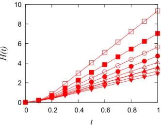
In all of the evolutions presented in this paper, the height seems to grow linearly fort≥0.3. Figure 3.1 presents the computed heightH(t) =H(t; 0) withρc ranging from 0.03 to 0.1. We denote byR△the growth rate obtained from least square approximation of the computed height in the time interval [0.3,1.0]. Table 1 shows some results comparing R△ to R(0). We observe that the normalized differences e(0) := |R
△−R(0)|/R(0) decrease at a rate which is larger than first order in ∆x.
Hereafter, we shall refer the above case (N = 1,m1 = 1,a1 = 0) or results
asa unit spiral case.
0 2 4 6 8 10
0 0.2 0.4 0.6 0.8 1
H
(t
)
t
Figure 3.1. Graphs ofH(t) for the evolution with a single screw dislocation and a unit spiral step. The holizontal axis
means time t. Each line with a mark means the case ρc =
Table 1. Normalized differencese(0)from numerical growth rates to the theoretical values by a unit screw dislocation.
e(0)
ρc s= 1 s= 2 s= 4 0.030 0.006807 0.004024 0.001630 0.040 0.005830 0.002902 0.001064 0.050 0.005093 0.002164 0.000738 0.060 0.004021 0.001619 0.000542 0.070 0.003464 0.001281 0.000395 0.080 0.002875 0.001056 0.000349 0.090 0.002585 0.001044 0.000428 0.100 0.002128 0.000665 0.000144
3.3. Co-rotating pair. In the following, we study the dynamics of
co-rotating pair of spirals and derive a new formula (3.7) for the growth rate for N co-rotating spirals. In Burton et al. [1], it is pointed out that the growth rate by a pair of co-rotating screw dislocations ata1and a2 depends
on the distance d := |a1 −a2| between the two screw dislocations. (Here
we have interpreted “activity of screw dislocations” in [1] by “growth rate” on the above. Hereafter, we similarly continue to use this interpretation.) More precisely,
(i) If the pair are far apart asd >2πρc =:dc, then the growth rate by the pair is indistinguishable from that of a unit spiral, i.e.,R(0).
(ii) If d≪ρc, then the growth rate should be twice of R(0).
On one hand they do not mention on between of the above situations, on the other hand they estimated the growth rate ofN co-rotating screw dis-locations on a line with lengthL as
(3.2) R(N)(L) = N
1 +L/(2πρc) R(0).
Our new formula gives a more accurate prediction of the critical distance separating the two cases mentioned above.
We first present a set of numerical simulations showing that the formula (3.2) is not accurate even forN = 2. Let
θ(x) = arg(x−a1) + arg(x−a2)
for a given pair a1 = (−α,0), a2 = (α,0) ∈ Ω with α > 0. Set u0 ≡ 0, so
that the initial steps are on the opposite line seguments of the line through
a1 and a2:
0 2 4 6 8 10 12 14 16 18
0 0.2 0.4 0.6 0.8 1
H
(t
)
t
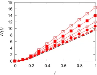
Figure 3.2. The left figure is the graphs of H(t) by a pair of co-rotating screw dislocations with ρc = 0.030. The line
with □ means the case of d := |a1−a2| = 0.04. Similarly, the line with■,◦, •, △, and ▲means the case of d= 0.08, 0.14, 0.20, 0.30 and 1.00, respectively. Note that the graphs with d= 0.30 andd= 1.00 are agree with each other. The dashed line isH(t) of the unit spiral with the sameρc.
Figure 3.2 shows the graphs ofHcomputed withρc = 0.03 in which we have 2πρc≈0.188496. From the Figure, we observe that the curves corresponding to d= 0.30 and 1.00 are very close to that computed from a single spiral. Furthermore, they are quite far from the curve corresponding to d = 0.2 (filled circles (•) in the figure). Since d = 0.2 is larger than 2πρc, the
numerical simulations suggest that the critical distance dc is larger than 2πρc. In fact, the fitting lines for d= 0.20,0.30,1.00 and the unit spiral for
ρc = 0.03 are
• d= 0.20: H(t)≈11.926788t−1.220501,
• d= 0.30: H(t)≈10.761760t−1.061625,
• d= 1.00: H(t)≈10.611018t−0.943661,
• unit: H(t)≈10.606435t−1.271220.
Miura and Kabayashi reported in [7] that they also found similar discrepancy using their phase field model. It is further pointed out, without providing an explicit formula, that the growth rate by a co-rotating pair is indistin-guishable from that of the unit spiral ifd≥3πρc.
(1) (2)
(3) (4)
Figure 3.3. Process of rotation of co-rotating spirals.
(i) The growth rate of a co-rotating pair with distanced=|a1−a2|is
given by
(3.3) R(2)(d) = 2h0
Td ,
where Td is the time that the pair of spiral steps goes rotating around the pair.
(ii) There are two fundamental motion during the rotation of co-rotating spirals: switching spirals (from (1) to (3) in Figure 3.3) and half turn (from (3) to (4) in Figure 3.3). Twice of the switchings and the half turns occur during the rotation once, and then
Td= 2(T1+T2),
where T1 and T2 is the time for the switching and the half turn. (iii) We regard the switching motion as the end point of spirals moves
from a1 toa2 with velocity v∞. Then,T1 =d/v∞.
(iv) In the half turn, the angular velocity should beω=ω1v∞/ρc. Then,
T2 =π/ω=πρc/(ω1v∞). (v) Consequently we obtain
Td= 2 (
d v∞
+ πρc
ω1v∞ )
= 2d+ 2πρc/ω1
v∞
By combining (3.3), (3.1) and the above we obtain
R(2)(d) = 2
1 +dω1/(πρc) ·
v∞ω1h0
2πρc =
2 1 +dω1/(πρc)
R(0).
Hence, for a pair of co-rotating spirals, we obtain the estimate of the growth rate
(3.4) R(2)(d) = 2
1 +dω1/(πρc)
R(0), ω1= 0.330958061,
where dis the distance between the two spiral centers which is assumed to be small. Furthermore, since R(2)(d)< R(0) ifd > πρ
c/ω1, the growth rate
with a co-rotating pair should be revised as
(3.5) R˜(2)(d) =
{
R(2)(d) ifd < πρc/ω1,
R(0) otherwise.
Consequently, the critical distance is revised to
(3.6) dc˜ = πρc
ω1
, ω1 = 0.330958061.
We remark that with ω1 = 1/2 the formulae (3.4) and (3.6) reduce to the
predictions in [1].
For verification we report the normalized differences
e(0)(d) := |R△(d)−R
(0)|
R(0) , e
(2)(d) := |R△(d)−R(2)(d)|
R(2)(d)
with respect to the distanced=|a1−a2|. Again,R△ computed by solving in (2.7) with the numerical data ont∈[0.3,1.0]. The numerical simulations are performed with the centers
a1 = (−k∆x,0), a2 = (k∆x,0) (2≤k≤50),
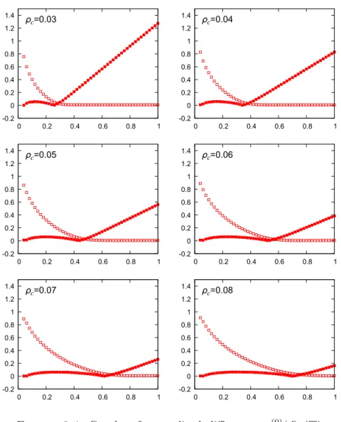
wheres= 1. Figure 3.4 presents numerical results ofe(0)(d) ande(2)(d). We observe that e(0)(d) is small ife(2)(d) is large, and inversely e(2)(d) is small
ife(0)(d) is large.
From the numerical results we also can define the numerical critical dis-tance ¯dc dividing the co-rotating pair and independent two single spirals as
¯
dc = sup{d; e(2)(d)< e(0)(d)}.
From Figure 3.4 it seems thate(0)(d) ande(2)(d) crosses only once in all the cases, so that we now calculate ¯dc with linear interpolation;
¯
dc ≈
Y1d¯k+Y0d¯k+1 Y1+Y0
,
where ¯k is such that e(2)(d¯
k) ≤ e(0)(d¯k) and e(2)(d¯k+1) > e(0)(d¯k+1) for dk= 2k∆x, and
Yj =|e(0)(d¯k+j)−e(2)(d¯k+j)|.
-0.2 0 0.2 0.4 0.6 0.8 1 1.2 1.4
0 0.2 0.4 0.6 0.8 1
=0.03
-0.2 0 0.2 0.4 0.6 0.8 1 1.2 1.4
0 0.2 0.4 0.6 0.8 1
=0.04
-0.2 0 0.2 0.4 0.6 0.8 1 1.2 1.4
0 0.2 0.4 0.6 0.8 1
=0.05
-0.2 0 0.2 0.4 0.6 0.8 1 1.2 1.4
0 0.2 0.4 0.6 0.8 1
=0.06
-0.2 0 0.2 0.4 0.6 0.8 1 1.2 1.4
0 0.2 0.4 0.6 0.8 1
=0.07
-0.2 0 0.2 0.4 0.6 0.8 1 1.2 1.4
0 0.2 0.4 0.6 0.8 1
=0.08
Figure 3.4. Graphs of normalized differences e(0)(d) (□) and e(2)(d) (■) for the pair a
1 = (−k∆x,0), a2 = (k∆x,0)
with respect to the distanced=|a1−a2|= 2k∆x.
Note that the estimate (3.4) is still rough in the sense that
edist= |
¯
dc−d˜c|
˜
dc
increase as ∆x decreases; see Table 3. On the other hand, one finds that
Table 2. Comparison of the critical distances: dc = 2πρc
used in [1], the revised distance ˜dc =πρc/ω1, and the
numer-ically observed critical distance ¯dc.
ρc 2πρc dc˜ dc¯
0.030 0.188496 0.284773 0.284813 0.040 0.251327 0.379697 0.379700 0.050 0.314159 0.474621 0.474650 0.060 0.376991 0.569545 0.569574 0.070 0.439823 0.664469 0.664486 0.080 0.502655 0.759394 0.759396
The numerical growth rates obtained in this subsection will be refered as
R△(2) in the following sections.
Table 3. Normalized differences of the critical distance be-tween ˜dc and ¯dc.
edist ρc s= 1 s= 2 0.030 0.000143 0.000275 0.040 0.000008 0.000013 0.050 0.000062 0.000108 0.060 0.000051 0.000094
3.4. Pair with opposite rotations. Consider the case that there is a
pair of unit screw dislocations with opposite rotation. Burton et al. [1] pointed out on this case as follows.
(i) Ifd=|a1−a2|<2ρc no growth occurs (calledinactive pair). (ii) If dis around 3ρc, then the growth rate is about 1.1×R0. (iii) Ifd→ ∞, then the growth rate decays exponentially toR0.
We shall verify the above speculations numerically; in particular, on the estimate of the growth rate with the case (ii) of the above and on the distance attaining the maximal growth rate.
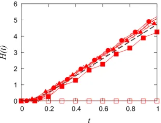
We first show the typical examples of the graphs of H(t) for pairs with opposite rotations in Figure 3.5. We present the numerical results using
d= 0.10<2ρc, with ρc = 0.06 on for case (i), d= 0.14 ∈(2ρc,3ρc) as the
case between (i) and (ii), d= 0.18 = 3ρc and d = 0.24 = 4ρc as (ii), and
0 1 2 3 4 5 6
0 0.2 0.4 0.6 0.8 1
H
(t
)
t
Figure 3.5. Graphs of H(t) for a pair with opposite
ro-tations with ρc = 0.06. Each graph means that d =
0.10 < 2ρc(□), d = 0.14 < 3ρc(■), d = 0.18 = 3ρc(◦),
d= 0.24 = 4ρc(•),d= 0.36(△) andd= 1.0(▲). The dashed line denotes the graph of H(t) on the unit case spiral with
ρc = 0.06.
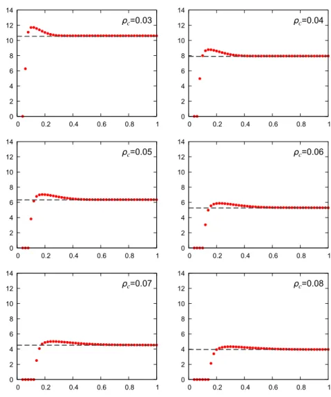
To clarify the relation between d = |a1 −a2| and R△, we numerically estimate the rates R△ for several ρc using computation performed in the
time interval [0.3,1.0]. In Fig 3.6 the red dots in each subplot correspond to
R△ computed with centers a1 = (−k∆x,0), a2 = (k∆x,0) for 2≤k ≤ 50
and ∆x= 0.01. Each subplot shows the computations using a different ρc. Thus, we observe that no growth occurs when d < 2ρc for the each case. By a similar argument as used in [12], one can prove that no growth would occur at the critical distanced= 2ρc. However, due to numerical errors, we observed slow growth at this critical distance from our computations. Our numerical simulations also show that, ifdis around 3ρc, the growth rate is larger than that corresponding to the unit spiral. In the subplots, the rate of the unit spiral is shown in the dashed lines.
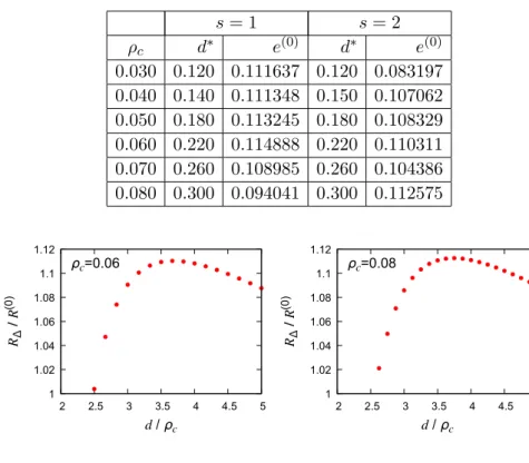
In the column for s = 1 in Table 4 we list the distance d∗ at which
the growth rate attains its maximum, and the normalized distance e(0) =
|R△−R(0)|/R(0) between R△ and R(0) at d = d∗. We find e(0) is around 0.1, and the maximum growth rate around 1.1×R(0), agreeing with [1] or [7]. However, we also find that the all results of d∗/ρc examined here are between 3.5 and 4, which are larger than that value described in [1] or [7]. See also Figure 3.7, which shows the relation betweenR△/R(0) andd/ρc for
ρc = 0.06 and 0.08 withs= 2.
3.5. Group on a line. In this section we consider a situation where
0 2 4 6 8 10 12 14
0 0.2 0.4 0.6 0.8 1
=0.03
0 2 4 6 8 10 12 14
0 0.2 0.4 0.6 0.8 1
=0.04
0 2 4 6 8 10 12 14
0 0.2 0.4 0.6 0.8 1
=0.05
0 2 4 6 8 10 12 14
0 0.2 0.4 0.6 0.8 1
=0.06
0 2 4 6 8 10 12 14
0 0.2 0.4 0.6 0.8 1
=0.07
0 2 4 6 8 10 12 14
0 0.2 0.4 0.6 0.8 1
=0.08
Figure 3.6. Graphs of R△ as a function of d = |a1−a2|.
The dashed line meansR(0) for the each case.
a line, i.e., there exists λj such that 0 = λ1 < λ2 < · · · < λN = 1 and aj = (1−λj)a1+λjaN. Burton et al. [1] estimated the growth rate by
such a a1, . . . , aN as (3.2) if |aj+1−aj|< dc for eachj = 1, . . . , N −1 and
|a1 −aN| = L. Then, by similar argument to obtain (3.4) as in §3.3, we
obtain the improved estimate of (3.2) as
(3.7) R(N)(d) = N
1 +Lω1/(πρc)
R(0), ω1 = 0.330958061.
Table 4. The distance between a pair of centers that result the maximal growth rate on a pair with opposite rotations.
s= 1 s= 2
ρc d∗ e(0) d∗ e(0)
0.030 0.120 0.111637 0.120 0.083197 0.040 0.140 0.111348 0.150 0.107062 0.050 0.180 0.113245 0.180 0.108329 0.060 0.220 0.114888 0.220 0.110311 0.070 0.260 0.108985 0.260 0.104386 0.080 0.300 0.094041 0.300 0.112575
1 1.02 1.04 1.06 1.08 1.1 1.12
2 2.5 3 3.5 4 4.5 5
=0.06
(0
)
/
1 1.02 1.04 1.06 1.08 1.1 1.12
2 2.5 3 3.5 4 4.5 5
=0.08
(0
)
/
Figure 3.7. Graphs showing relation betweenR∆/R(0) and
d/ρc forρc = 0.06 and 0.08 withs= 2.
of the above formula and presented numerical simulations for several co-rotating screw dislocations (N ≥2) withω1 = 2π/19 and equally arranged
dislocations. However, actually the distribution of screw dislocations has influence to the growth rate. We present below numerical results verifying this assertion.
Consider the situation N = 3 and ˜dc <|a1−a3|<2 ˜dc, for example,
(3.8) a1= (−0.35,0), a2= (−k∆x,0), a3 = (0.35,0)
with ρc = 0.05 for k ≥ 0. Note that the critical distance ˜dc = 0.474650 is
less than distance between the two farthest center L = |a1 −a3| = 0.70.
Here we have used the revised critical distance as presented in§3.3. In this case, the situations are divided into the following two situations.
(a) A group of triplets, if|a2−a3| ≤d˜c,
(b) A co-rotating pair and independent unit spiral, if |a2−a3|>d˜c.
by [1] were valid, the growth rate by this group with respect to |a1−a2|
would have a unnatural discontinuity at |a1−a2|=L−dc˜ as in left figure of Figure 3.8. Hence, we examine the growth rate of triplets at (3.8) with
ρc = 0.05, aiming at revealing whether or not such a discontinuity appears.
Our results are presented in the right plot in Figure 3.8.
7 7.5 8 8.5 9 9.5 10 10.5 11
0.1 0.15 0.2 0.25 0.3 0.35 7 7.5 8 8.5 9 9.5 10 10.5 11
0.1 0.15 0.2 0.25 0.3 0.35 7 7.5 8 8.5 9 9.5 10 10.5 11
0.1 0.15 0.2 0.25 0.3 0.35 7 7.5 8 8.5 9 9.5 10 10.5 11
0.1 0.15 0.2 0.25 0.3 0.35
Figure 3.8. Comparison between estimates by [1] (left
fig-ure) and numerical simulations (right figfig-ure) withρc = 0.05.
The horizontal axis corresponds to |a1−a2|and the vertical
axis is the rate. The dashed vertical line shows the distance
|a1−a2|= 0.70−dc˜ (i.e.,|a2−a3|= ˜dc) withρc = 0.05. The dashed horizontal line shows the rate R(3)(0.70)≈7.662046
given by (3.7). The chain line and the dotted line denote
R(2) (left figure) andR(2)△ obtained in §3.3, respectively.
The right figure in Figure 3.8 presents numerical results of the growth rate by (3.8) with ρc = 0.05 for 0≤k≤25 with respect tod:=|a1−a2|=
0.35−k∆x. The growth rates are estimated in the time interval [0.3,1.0]. We also plot R△(2)(|a1 −a2|) as the dotted line. The growth rates of the
triplets follows closely the values of R(2)△ (|a1 − a2|) on the region where
R△(2)(|a1 −a2|) > R(3)(L) even if the centers are sufficiently close to be
regarded as the group in the sense of [1] (to the right of the dashed vertical line). However, whenR(2)△ becomes smaller thanR(3)(0.70) (indicated by the dashed horizontal line), the growth rate of the triplets becomes larger than
R△(2). Results similar to the above are obtained with the following setups: (i) ρc = 0.06, a1 = (−0.35,0), a2 = (−k∆x,0), a3 = (0.35,0) for
−25≤k≤0,
(ii) ρc = 0.05, a1 = (−0.40,0), a2 = (−k∆x,0), a3 = (0.40,0) for −30≤k≤0.
See Figure 3.9.
6 6.5 7 7.5 8 8.5 9
0.1 0.15 0.2 0.25 0.3 0.35
6 6.5 7 7.5 8 8.5 9
0.1 0.15 0.2 0.25 0.3 0.35
6 6.5 7 7.5 8 8.5 9
0.1 0.15 0.2 0.25 0.3 0.35
6 6.5 7 7.5 8 8.5 9
0.1 0.15 0.2 0.25 0.3 0.35
6.5 7 7.5 8 8.5 9 9.5 10
0.1 0.15 0.2 0.25 0.3 0.35 0.4 6.5 7 7.5 8 8.5 9 9.5 10
0.1 0.15 0.2 0.25 0.3 0.35 0.4 6.5 7 7.5 8 8.5 9 9.5 10
0.1 0.15 0.2 0.25 0.3 0.35 0.4 6.5 7 7.5 8 8.5 9 9.5 10
0.1 0.15 0.2 0.25 0.3 0.35 0.4
Figure 3.9. Growth rates of the triplets with case (i) and
(ii). The holizontal and vertical dashed line respectively de-notes R(3)(L) and|a
1−a2|=L−dc˜ for each cases.
in Figure 3.10. Note that we chooses= 1, i.e., ∆x= 0.01 for the consistency of numerical results, but we calculate R2△(d) with the linear interpolation for d = 0.11,0.13, . . . ,0.35. One can find that the growth rates are quite separated fromR(2)△ ifdis larger than where R(2)△ goes acrossR(3)(L).
In the simulations with case (i), note that the triplets should be regarded as a co-rotating group of triplet ifk ≤21 (|a2−a3| ≤ 0.56). However, the
growth rate becomes quite larger than that by a co-rotating pair if k≤13, where R2(d) is also smaller than R3(0.7) with ρc = 0.06 if d≥ 0.22. The case (ii) also proposes that the growth rates become faster than those by a co-rotating pair provided thatk≤6 although the triplets should be regarded as a co-rotating group of triplet ifk≤2 (|a2−a3| ≤0.38). One can find in
the both cases that the growth rate by a co-rotating triplet is faster than a co-rotating pair, however, slower than that calculated by (3.7).
From our numerical simulations, we have the following predictions (note that the quantities are simulations by (3.8) with ρc = 0.05):
• The growth rate seems to decay smoothly ford≥0.23 although the triplets are classified as a group if 0.23≤d≤0.35.
• The growth rate by the triplets becomes smaller than R(3)(0.70) if
d ≥0.27, however it continues to decay. Note that R(2)△ (d) is also smaller than R(3)(0.70) ifd≥0.27.
0 0.02 0.04 0.06 0.08 0.1
0.1 0.15 0.2 0.25 0.3 0.35 0 0.02 0.04 0.06 0.08 0.1
0.1 0.15 0.2 0.25 0.3 0.35 0 0.02 0.04 0.06 0.08 0.1
0.1 0.15 0.2 0.25 0.3 0.35 0 0.02 0.04 0.06 0.08 0.1
0.1 0.15 0.2 0.25 0.3 0.35 0 0.02 0.04 0.06 0.08 0.1
0.1 0.15 0.2 0.25 0.3 0.35 0 0.02 0.04 0.06 0.08 0.1
0.1 0.15 0.2 0.25 0.3 0.35 0 0.02 0.04 0.06 0.08 0.1
0.1 0.15 0.2 0.25 0.3 0.35 0 0.02 0.04 0.06 0.08 0.1
0.1 0.15 0.2 0.25 0.3 0.35 0 0.02 0.04 0.06 0.08 0.1
0.1 0.15 0.2 0.25 0.3 0.35 0.4 0 0.02 0.04 0.06 0.08 0.1
0.1 0.15 0.2 0.25 0.3 0.35 0.4 0 0.02 0.04 0.06 0.08 0.1
0.1 0.15 0.2 0.25 0.3 0.35 0.4 0 0.02 0.04 0.06 0.08 0.1
0.1 0.15 0.2 0.25 0.3 0.35 0.4
Figure 3.10. Normalized distances |R△(d) −
R(2)△ (d)|/R(2)(d) with ρc = 0.05, L = 0.7, ρc = 0.06,
L = 0.7, and ρc = 0.05, L = 0.8, respectively. The dashed lines are at L−d˜c, and the solid lines at |a1 −a2| = 0.265
(top), 0.225 (middle) or 0.335 (bottom) approximately denote the distance where R(2)△ goes across R(3)(L) in each cases.
As supplementary evidences to the above assertion, we present some ex-amples of calculation of the growth rates for 4 co-rotating screw dislocations as in [9]. Recall the situation of the simulations: 4 co-rotating screw dislo-cations are located at
a1= (−a,0), a2= (−b,0), a3= (b,0), a4 = (a,0)
with
(a) a= 0.06 andb= 0.02, (b) a= 0.15 andb= 0.11.
The evolution equation is
i.e., v∞= 5 and ρc = 0.02. We choose the initial steps as
a1 : {a1+ (−r,0); r >0}, a2 : {a2+ (0,−r); r >0}, a3 : {a3+ (0, r); r >0}, a4 : {a4+ (r,0); r >0}.
See [9] for the details of the initial data, and the profiles of spiral steps at
t= 0.5. Profiles are slightly different from each other. We now give a clas-sification if these situations are a group of 4 co-rotating screw dislocations, or 2 pairs from a view point of the growth rates. See Figure 3.11 for the
0 5 10 15 20 25 30
0 0.2 0.4 0.6 0.8 1
0 5 10 15 20 25 30
0 0.2 0.4 0.6 0.8 1
Figure 3.11. Graphs of H(t) by 4 screw dislocations
(a)(±0.06,0) and (±0.02,0)(left), or (b)(±0.15,0) and (±0,11,0)(right). The points denote the data of H(t) per the time span ∆t = 0.05, and solid lines denote the fitting line by the data of H(t) in [0.3,1].
data plots ofH(t) on these simulations. Each fitting line is as follows;
(a) H(t)≈31.96154528t−4.26148724, (b) H(t)≈21.29516137t−2.33023461.
Then, the growth rate of the case (a) is R△,1 = 31.96154528, and that of
the case (b) is R△,2 = 21.29516137. The growth rate R(0) with v∞ = 5,
ρc = 0.02 is
R(0) = 5ω1
0.04π ≈13.168403.
The possibility of the classification (a) is
(a1) a group of{a1, a2, a3, a4} with lengthL= 0.12, (a2) a group of{a1, a2, a3} and an independent{a4},
Then, each growth rate is calculated as follows.
(a1) R(4)(0.12) = 4
1 + 0.12ω1/(0.02π)R
(0) ≈32.273849,
(a2) R(3)(0.08) = 3
1 + 0.08ω1/(0.02π)
R(0) ≈27.793385,
(a3) R:= 2
1 + 0.08ω1/(0.02π)
R(2)(0.04)≈30.608752.
For case (a) one can find R(4)(0.12) is the closest to R△,1. So case
(a) should be regarded as a group of four co-rotating screw dislocations. Case (b), on the other hand, should be regarded as two independent (non-interacting) pairs {a1, a2} and {a3, a4} since a2 and a3 are disconnected
in the sense that |a2 −a3| = 0.22 > dc˜. Thus, the growth rate should
be estimated as R(2)(0.04) ≈ 21.753470. Even if we regard case (b) as a group of four screw dislocations on a line of length 0.30, (3.7) gives
R(4)(0.30) ≈ 20.414480, which is farther than R(2)(0.04). Similarly, if we treat{a1, a2} and{a3, a4} as two effective pairs of centers, we obtain
R= 2
1 + 0.26ω1/(0.02π)R
(2)(0.04)
≈18.361125
by calculation similar to (a3). Note that the centers of the pair in this case should be regarded as (±0.13,0).
3.6. Complex group. According to [1] the growth rate of crystal surface
by several screw dislocations, could be estimated systematically by analyz-ing groups of screw dislocations independently. In essence, dislocations are collected into disjoint subsets. We shall refer to each of such subsets as a group. Inactive pairs are discarded from the groups. In each group, any dis-location center is no farther thandc distance away from another dislocation center in the same group. Each group can be assigned a strengthn, which is defined as
n=n+−n−,
wheren+ orn− are number of single screw dislocations which has counter-clockwise or counter-clockwise rotational orientations provided that the steps evolve, respectively. By the signed number mj of screw dislocations defined as in
§2.1 or [9], we represent nas
n=∑
j∈Λ mj,
where Λ is the set of numbers of screw dislocations in the group. It is mentioned in [1] that ifn= 0, then the growth rate by the group is approx-imately the same as that of the unit spiral; otherwise, n ̸= 0, the growth rate is|n|times that of the unit spiral.
of these effective growth rates. Of course, in our analysis, we use the revised critical distance ˜dc as defined in (3.6) for grouping the centers.
Motivated by the above speculation, we study numerically the growth rates of a surface consisting of two groups of dislocations which are getting closer in distance. In particular, we consider the case in which one the groups consist of a single dislocation. For example, we consider the evolution of the surface with
(3.9) a1 = (0,−0.05; 1), a2 = (0,0.05; 1), a3 = (k∆x,0;−1) fork≥0
with the evolution equation
(3.10) V = 6(1−0.04κ),
i.e., v∞ = 6, ρc = 0.04. In (3.9), we have expressed the screw dislocation aj as the triplet (pj, qj;mj) where (pj, qj) is the coordinates of dislocation, and mj ∈ {±1} is the rotational orientation. By [1] the growth rate can be
estimated by:
(c1) If|a1−a3| ≥dc˜, the growth rate should be max{R(2)(0.10), R(0)}=
R(2)(0.10) withρc = 0.04.
(c2) If 2ρc ≤ |a1−a3|<dc˜, then {a1, a2, a3} are all in the same group
ands= 1 on this group. The growth rate should be 1×R(0) =R(0).
(c3) If|a1−a3|<2ρc := 0.08, thena1 and a3 form an inactive pair, and
only a2 influences the growth rate. The growth rate should beR(0).
Note that in this case |a1 −a3|=
√
0.052+ (k∆x)2, so that the first case
appears when
k∆x≥a∗∗:= √
˜
d2
c −0.052 ≈0.376390,
and the third case appears when
k∆x=a∗:=√(2ρc)2−0.052 ≈0.062450.
Hence, we obtain the estimate of the growth rate by (3.9) as in the top-left figure of Figure 3.12. For this speculations, our interests in this section are as follows.
(i) Why the effective distance is ˜dc even for pair of screw dislocations with opposite rotational orientations? The effective line between the pair with opposite rotational orientations should be shorter than 2ρc.
(ii) Dependency of the length of effective line to the growth rate. We think the discontinuity as shown in Figure 3.12 is unnatural. The top-right figure in Figure 3.12 shows the graph of the numerical growth rateR△in this situation, which is calculated on a time interval [0.7,2.0]. The holizontal axis means k∆x. The holizontal dashed lines in the right figure are drawn at R(0) ≈ 7.901042 and R(2)
6 7 8 9 10 11 12 13 14
0 0.1 0.2 0.3 0.4 0.5
6 7 8 9 10 11 12 13 14
0 0.1 0.2 0.3 0.4 0.5
6 7 8 9 10 11 12 13 14
0 0.1 0.2 0.3 0.4 0.5
6 7 8 9 10 11 12 13 14
0 0.1 0.2 0.3 0.4 0.5
6 7 8 9 10 11 12 13 14
0 0.1 0.2 0.3 0.4 0.5
6 7 8 9 10 11 12 13 14
0 0.1 0.2 0.3 0.4 0.5
6 7 8 9 10 11 12 13 14
0 0.1 0.2 0.3 0.4 0.5
6 7 8 9 10 11 12 13 14
0 0.1 0.2 0.3 0.4 0.5
6 7 8 9 10 11 12 13 14
0 0.1 0.2 0.3 0.4 0.5
6 7 8 9 10 11 12 13 14
0 0.1 0.2 0.3 0.4 0.5
6 7 8 9 10 11 12 13 14
0 0.1 0.2 0.3 0.4 0.5
11.8 11.9 12
0 0.1 0.2 0.3 0.4 0.5
11.8 11.9 12
0 0.1 0.2 0.3 0.4 0.5
11.8 11.9 12
0 0.1 0.2 0.3 0.4 0.5
11.8 11.9 12
0 0.1 0.2 0.3 0.4 0.5
11.8 11.9 12
0 0.1 0.2 0.3 0.4 0.5
Figure 3.12. The estimate by [1] of the growth rate by (3.9) (top-left) and its numerical results(top-right). The horizontal axis means k∆x, and the vertical dashed line are located at
k∆x = a∗ or a∗∗. In the bottom figure, we zoom in the numerical results around 11.9 of y-axis.
0 5 10 15 20 25
0 0.5 1 1.5 2
0 5 10 15 20 25
0 0.5 1 1.5 2
0 5 10 15 20 25
0 0.5 1 1.5 2
Figure 3.13. Graphs ofH(t) and profiles of spirals att= 2 with s = 1 (∆x = 0.01) for each case of (c1), (c2), (c3) as
In Figure 3.13 we present three numerical simulations, usingk= 40,10,5 corresponding to cases (c1)–(c3). The numerically observed growth rates are
R△ = 6.863008, R△ = 11.064736, R△= 11.860357. On the other hand, we have
R(0)≈7.901042, R(2)(0.10)≈12.507902, R(2)△ (0.10)≈11.904457,
where R(2)(0.10) is calculated with (3.4), and R(2)△ (0.10) is the numerical result obtained in §3.3. There seem to be quite some discrepancy between the presented computation and the one predicted by [1].
We now summarize the numerical results in Figure 3.12 as follows.
• The growth rate keeps its quantity around R△(2)(|a1 −a2|) until
k∆x ≥ 0.15. Note that |a1 −a3| ≈ 0.158114 for k∆x = 0.15 is
close to 4ρc = 0.16.
• The growth rate is smaller than R(0) if|a1−a3|<2ρc.
• The growth rate attains its maximum at 2ρc < |a1 −a3| < dc˜,
and monotone decrease for|a1−a3|over the distance achieving the
maximal growth rate.
The profile of the growth rate at |a1 −a3|>2ρc looks like the subplots in Figure 3.6. So, similar overshooting of growth rates as a pair with opposite rotational orientation may appear if a group includes an accelerating pair with opposite rotations. On the other hand, the second fact of the above implies that an inactive pair in a group of screw dislocations may reduce the growth rate of the group.
In this section, the growth of surface by a triplet with co-rotating pair and other one having opposite rotational orientation is examined. In the numer-ical simulations, we fix a co-rotating pair of spirals, and study the growth rate as the center of the third spiral, with opposite rotational orientation, approaches the former two. We observed that if the distance, L, between center of the third spiral and those of the co-rotating ones is larger than the critical distance (for an inactive pair of spirals), then the growth rate tends rapidly to the rate of the co-rotating pair, as L becomes larger. IfL is too small, then the growth rate is less than that of the unit spiral.
4. Conclusion and remarks
(of co-rotating pair) with the view point of effective growth rate. We also gave an improved estimate of the growth rate by a co-rotating pair with a estimate of the rotating single spiral by Ohara-Reid [8]. By arguments used in the above two items, we concluded that the critical distance by [1] is too small. We found that the growth rate by a pair of opposite rotational screw dislocations, attains the maximum with the distance between the spi-ral centers is between 3.5ρc and 4ρc. We found that the distribution of screw
dislocations on a line influences to the growth rate. We carefully studied how the growth rate depends on the distribution. For general group of spirals, we found that the growth rate can be studied systematically by the rates of the ”effective” sub-groups of centers, partitioned by the inter-distances.
References
[1] W. K. Burton, N. Cabrera, and F. C. Frank. The growth of crystals and the equi-librium structure of their surfaces.Philosophical Transactions of the Royal Society of London. Series A. Mathematical and Physical Sciences, 243:299–358, 1951.
[2] N. Cabrera and M. M. Levine. Xlv. on the dislocation theory of evaporation of crys-tals.Philosophical Magazine, 1(5):450–458, 1956.
[3] Yoshikazu Giga. Surface evolution equations: A level set approach, volume 99 of
Monographs in Mathematics. Birkh¨auser Verlag, Basel, 2006.
[4] Shun’ichi Goto, Maki Nakagawa, and Takeshi Ohtsuka. Uniqueness and existence of generalized motion for spiral crystal growth.Indiana University Mathematics Journal, 57(5):2571–2599, 2008.
[5] Alain Karma and Mathis Plapp. Spiral surface growth without desorption.Phys. Rev. Lett., 81:4444–4447, Nov 1998.
[6] Ryo Kobayashi. A brief introduction to phase field method. AIP Conf. Proc., 1270:282–291, 2010.
[7] Hitoshi Miura and Ryo Kobayashi. Phase-field modeling of step dynamics on growing crystal surface: Direct integration of growth units to step front. Crystal Growth & Design, 15(5):2165–2175, 2015.
[8] M. Ohara and R. C. Reid.Modeling Crystal growth rates from solution. Prentice-Hall Inc., 1973.
[9] T. Ohtsuka, Y.-H.R. Tsai, and Y. Giga. A level set approach reflecting sheet struc-ture with single auxiliary function for evolving spirals on crystal surfaces.Journal of Scientific Computing, 62(3):831–874, 2015.
[10] Takeshi Ohtsuka. A level set method for spiral crystal growth.Advances in Mathe-matical Sciences and Applications, 13(1):225–248, 2003.
[11] Takeshi Ohtsuka. Evolution of crystal surface by a single screw dislocation with mul-tiple spiral steps.S¯urikaisekikenky¯usho K¯oky¯uroku, (1924):11–20, 2014. Mathematical analysis of pattern formation arising in nonlinear phenomena (Kyoto, 2013). [12] Takeshi Ohtsuka. Inactive pair in evolution of an opposite rotating pair of spirals by
eikonal-curvature flow equations. in preparation.
[13] Stanley Osher and Ronald P. Fedkiw. Level set methods: an overview and some recent results.J. Comput. Phys., 169(2):463–502, 2001.
[14] Stanley Osher and James A. Sethian. Fronts propagating with curvature-dependent speed: algorithms based on Hamilton-Jacobi formulations. J. Comput. Phys., 79(1):12–49, 1988.
4-2, Aramaki-machi, Maebashi, Gunma 371-8510, Japan
The University of Texas at Austin, USA and KTH Royal Institute of Tech-nology, Sweden

![Table 2. Comparison of the critical distances: d c = 2πρ c used in [1], the revised distance ˜d c = πρ c /ω 1 , and the numer-ically observed critical distance ¯d c .](https://thumb-ap.123doks.com/thumbv2/123deta/9836677.489926/13.892.354.562.554.689/comparison-critical-distances-revised-distance-observed-critical-distance.webp)
![Figure 3.8. Comparison between estimates by [1] (left fig- fig-ure) and numerical simulations (right figfig-ure) with ρ c = 0.05](https://thumb-ap.123doks.com/thumbv2/123deta/9836677.489926/17.892.229.698.298.476/figure-comparison-estimates-left-numerical-simulations-right-figfig.webp)
