Quality Sorting, Alchian‑Allen Effect, and Geography
著者 TAKECHI Kazutaka
出版者 Institute of Comparative Economic Studies, Hosei University
journal or
publication title
Working Paper
volume 214
page range 1‑28
year 2019‑01‑29
URL http://hdl.handle.net/10114/00022486
Quality Sorting, Alchian–Allen Effect, and Geography
Kazutaka Takechi∗
Faculty of Economics Hosei University 4342 Aihara-machi
Machida, Tokyo, 194-0298, Japan Email: [email protected]
Abstract
The positive relationship between product quality and the distance to market is generally considered evidence of either quality sorting or the presence of a specific cost (the so-called Alchian–Allen effect). However, reduced-form regressions using free-on-board (FOB) prices do not reveal which of these two mechanisms is the primary driver. In this study, we employ unique Japanese individual goods price data to separately identify the effects of quality sorting and specific costs. Our empirical analysis shows that high-cost producers produce high-quality goods as quality sorting suggests.
However, the empirical results are inconsistent with a model where only quality sorting exists, but are consistent with one that also includes specific costs. We also find that the specific cost component in trade costs is more distance elastic than the ad valorem component. Our results are robust with respect to various measures of distance and specification.
Key Words: Quality sorting; Trade costs; Specific costs; Geographic barriers JEL Classification Number : F11, F14, F41
Date: January 28, 2019
∗ The author would like to thank Taiji Furusawa, Jota Ishikawa, Volodymyr Lugovskyy, Andreas Moxnes, Kentato Nakajima, and Ryosuke Okamoto for useful discussions. The author also thanks seminar participants at the spring meeting of the Japan Society of International Economics, the National Graduate Institute for Policy Studies, Hosei University, the Research Institute of Economy, Trade and Industry (RIETI), and the University of British Columbia for their useful comments and suggestions. The usual disclaimer applies. The author gratefully acknowledges the financial support of the Ministry of Science, Technology and Education (Grant No. 18K01624). This study was conducted as a part of the Trade and Industrial Policies in a Complex World Economy project undertaken at RIETI.
1. Introduction
Are the markets for high-quality goods more remote than those for low-quality goods?
The response of many studies appears to be in the affirmative (Bastos and Silva (2010), Baldwin and Harrigan (2011), Manova and Zhang (2012), Martin (2012)). While this positive relationship between the quality of goods and the distance to market results only from simple observation, it does lead to a more primary concern when evaluating trade models and the specification of trade costs. This is because such an empirical relationship is inconsistent with the prediction of standard firm-heterogeneity models in the absence of a quality dimension and the specification of iceberg- type trade costs. Therefore, to reconcile the available empirical and theoretical evidence, we need to incorporate the form of quality sorting and the presence of specific trade costs into our modeling.
A quality-sorting mechanism implies the supply of high-quality goods to high trade cost markets. Because high-quality products are also highly profitable, and normally highly priced, they can overcome the significant trade costs associated with long distances to market. When measuring quality based on the average free-on-board (FOB) price, the observed price is typically high in remote markets. In contrast, in standard productivity–heterogeneity trade models, as distance increases, only highly productive, and hence low-cost firms, can provide supply. Because low-cost producers are able to set lower prices, the FOB price is lower in distant markets, which is not what the pattern of observed data suggests. Hence, it is necessary to incorporate quality in a firm-heterogeneity model to account for the supposed positive relationship between it and distance (Baldwin and Harrigan, 2011).
The presence of specific costs also accounts for the positive relationship between good quality and distance to market. The relative prices of high quality, and therefore higher-priced, goods are lower in distant markets when there are specific costs in trade. Hence, the relative demand for high-quality goods is also high in these markets. This enables firms producing high-quality goods to ship to these more distant markets, a process referred to as the Alchian–Allen effect (Hummels and Skiba, 2004). Importantly, this change in relative prices does not arise under iceberg-type trade costs.
However, largely because of data limitations, to our knowledge the Alchian–Allen and quality-sorting effects have not been jointly analyzed using individual pricing data. In the lit- erature, the FOB price (the unit value) of export goods is regressed on the distance to market.
Problematically, the positive relationship typically identified is driven by either the presence of specific costs or the situation where high-quality goods overcome the cost penalty associated with long distances to markets. Thus, we require a trade cost specification that consists of ad valorem and specific elements. In the absence of trade cost data and the proper specification of the trade cost function, we would be unable to correctly attribute variations in quality to distance. With the exception of Hummels (2001) and Hummels and Skiba (2004), such identification remains as yet incomplete because trade cost information is invariably unavailable and specific cost is not
included. The contribution of this study to the literature is then to analyze the quality-sorting and Alchian–Allen effects jointly and to identify these effects separately.
In the recent literature, several studies incorporate specific cost components in trade costs and assess their size and impact. For instance, Irarrazabal et al. (2015) show that the size of specific costs is large and significant, while Khandelwal et al. (2013) use specific costs to model quotas, which affect firm behavior differently to an ad valorem cost reduction. While our analysis shares a common motivation concerning the impact of specific costs, our focus is slightly different in being the identification of the impact of distance on ad valorem and specific costs. We argue that if the effect of distance on specific costs is large, a framework excluding specific costs may be severely misspecified.
In this paper, we first follow Anderson and van Wincoop’s (2004) suggestion for use of the price of production (at the source or origin). The use of source and market price data enables us to measure trade costs because there is actual delivery between these areas. As examples of the use of origin information, Donaldson (2018) uses salt price data in India while Atkin and Donaldson (2015) employ price data in Ethiopia, Nigeria, and the United States (for which source prices are also available). Elsewhere, Kano et al. (2013) specify wholesale vegetable price data in Japan, including a detailed description that allows for the identification of identical products in different locations. Because price differentials reflect both ad valorem and specific costs, it remains necessary to identify these costs separately. Then, our strategy is again using origin price. By utilizing the optimal price formula, we are able to obtain information on production costs from the price data.
Moreover, while price differentials are linear in ad valorem trade cost terms, there is an interaction term in the form of specific trade costs multiplied by production costs. Hence, the production costs derived enable us to separate ad valorem costs from specific costs.
There is also an additional identification problem in that if shipping is too costly, producers may not even supply high-quality goods to distant markets. This self-selection bias is absent in most of the literature, with the exception of Helpman et al. (2008), Johnson (2012) and Kano et al.
(2013, 2014). To overcome this, we employ unique micro data on agricultural product (vegetable) prices in Japan. As in Kano et al. (2013, 2014), this data set contains market and origin prices, as well as information on the region where a product is produced. Thus, we can establish product delivery patterns and consider the selection bias arising from delivery choices.
The analysis in this paper begins with reduced-form regressions as in the existing literature.
Our origin price is approximately equivalent to the FOB price in this literature used to measure product quality. Therefore, we first simply regress origin prices on the distance to markets and find that our vegetable qualities are, as in the literature, also positively associated with the distance to market. We then estimate a structural model to obtain the ad valorem and specific cost components separately. We use the origin price and markup formula to back out the cost of production and utilize the derived production cost to identify the ad valorem and specific costs.
The empirical analysis shows that the technology parameter connecting production costs
and quality is positive: high-cost producers produce high-quality goods as suggested by Baldwin and Harrigan (2011). However, the empirical results are inconsistent with a model where only quality sorting exists, but are consistent with one that also includes specific costs. That is, the magnitude of the increase in quality associated with production costs is too low under an iceberg- type specification to account for the positive link between quality and distance. This suggests that while there is a quality-sorting mechanism, we need the model with specific costs to obtain consistent empirical results. Our estimations also show that the specific cost component is more distance elastic than the ad valorem component, which is qualitatively consistent with the specification in Hummels and Skiba (2004). In addition, the size of the technology parameter with no specific costs is higher than with specific costs. That is, without specific costs, we could overestimate the rate of quality improvement by incurring cost. Thus, our contribution is not only to detect properly the relationship between quality and distance, but also to correctly identify the technical relationship between quality and production costs.
Existing studies such as Irarrazabal et al. (2015) have also identified the significance of specific costs. The identification strategy in Irarrazabal et al. (2015) is to utilize the property that the presence of specific costs changes the demand elasticity. To identify this, Irarrazabal et al. (2015) estimate the size of the specific costs relative to the ad valorem costs using the data variation in FOB (producer) prices and destinations (trade costs). Our study is notable in that we estimate the ad valorem and specific components separately and then identify how these costs are sensitive to distance. Additionally, we also estimate the elasticity of substitution parameters and thus obtain the key parameters in the heterogeneous-quality model, including the quality elasticity with respect to production costs, the elasticity of substitution, and the distance elasticity. As these determine the behavior of the heterogeneity model, our estimates yield a benchmark for evaluating the implications of existing theoretical models.
Of course, our results relate in part to the characteristics of the data employed. In particular, we use price data for agricultural products. Thus, the reason for the rather weak effect of quality sorting in our analysis is that vegetable production is constrained by geographic conditions. While some farmers may produce high-quality goods using superior technology (e.g., greenhouses), farmer productivity is generally associated with costs not quality. Thus, the demand side may matter more.
Specific costs make the price of high-quality goods relatively lower, thereby creating relatively high demand in remote markets. Hence, the presence of specific costs in our model encourages farmers able to produce high-quality goods to deliver their products to distant markets. In addition, because of the use of domestic data, transport costs represent the major part of trade costs and these largely depend on quantity, not the value of goods. This may contribute to a large distance-elastic specific cost.
The remainder of the paper is as follows. In Section 2, we discuss the reduced-form re- gressions representing the relationship between quality and distance. In Section 3, we set up a structural model for our estimations. For clarifying our argument on reduced-form analysis and
building a structural model, we conduct Monte Carlo exercises to reveal the identification issues and demonstrate the bias in the standard model in Section 4. Section 5 introduces our data set, and Section 6 details the specification of our model. Section 7 reports the estimation results, and Section 8 provides some robustness checks. In Section 9, we evaluate the welfare improvements associated with the reduction in trade costs using general equilibrium model simulations. The final section provides some concluding remarks.
2. Quality and Origin Price
It is often difficult to measure the quality of products. This is because quality measure data are not readily available for most goods (and a certain level of aggregation suffers from the composition of goods with different-level qualities) and it is not obvious what characteristics of goods are valued most highly by consumers (e.g., high-powered or fuel-efficient cars). It is rare that a particular measure of quality represents the quality of goods properly (Crozet et al.
(2012)). As discussed in detail later, our data set is price data from vegetable wholesale markets and these data contain detailed information about several product characteristics, including size and grade. However, because of the unobservable nature of product quality and seasonality, our product characteristics are not sufficient to capture the quality of goods. This is important because unobservable product quality may contribute to the price differences between goods sharing the same product characteristics. For example, on May 2, 2007, two bulk lots of cabbages produced in Aichi Prefecture with size “L” and grade “excellent” traded in the Aichi market. While these product characteristics are identical, the average prices of the cabbages per kilogram (kg) were 124.6 and 138.3 yen, respectively. This ten percent price difference could be attributed to unobservable factors.1 Therefore, we adopt an approach taken by the trade literature, which is that the price in origin (often the FOB price) serves as a proxy for product quality. If the origin price is high, it then reflects high-quality goods.
The importance of the origin price information for product quality can be also shown by the link between market price and product characteristics, such as the size and grade of goods and the origin price. If the origin price is a significant factor for the market price, even after incorporating goods characteristics, it likely captures certain aspects of unobservable quality. Thus, we regress market prices on the index of high quality, that of large size, and the origin price. In addition, because the origin price for goods shipped locally is identical to the market price, we use only that sample of goods shipped to different regions. We identify the product characteristics using the name of the characteristics, such that a grade name including “syu” (excellent) indicates that the product is high quality and a size category including the letter “L” designates a large size. We construct
1With respect to seasonality, cabbages produced in Aomori prefecture with size “L” and grade “A” traded in the Aomori market from July 2007 to November 2007. Once again, the product characteristics were the same, but the prices were 73.5, 105.0, 78.8, 63.0, and 57.8 on July 13, August 7, September 14, October 3, and November 5, respectively.
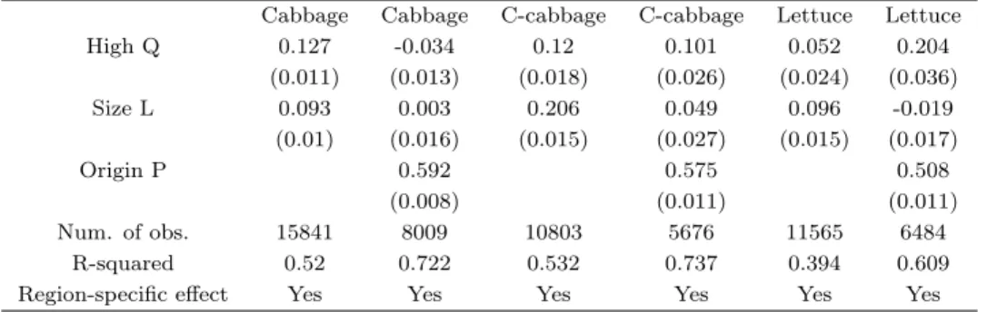
an index variable such that the high quality index takes a value of one if the grade characteristics include the name ”excellent” and zero otherwise, and the large size index takes a value of one if the size category is equal to or larger than size ”L” (such as “2L”) and zero otherwise. Table 1 reports that origin prices are significantly positive after controlling for product characteristics, which implies that the origin price captures an important element of product quality. We turn to
Cabbage Cabbage C-cabbage C-cabbage Lettuce Lettuce
High Q 0.127 -0.034 0.12 0.101 0.052 0.204
(0.011) (0.013) (0.018) (0.026) (0.024) (0.036)
Size L 0.093 0.003 0.206 0.049 0.096 -0.019
(0.01) (0.016) (0.015) (0.027) (0.015) (0.017)
Origin P 0.592 0.575 0.508
(0.008) (0.011) (0.011)
Num. of obs. 15841 8009 10803 5676 11565 6484
R-squared 0.52 0.722 0.532 0.737 0.394 0.609
Region-specific effect Yes Yes Yes Yes Yes Yes
Table 1: The Relationship between Market Prices and Product Characteristics
the key relationship between the origin price and the distance to market. A positive relationship between FOB prices and distance has been obtained in a number of previous studies, including Bastos and Silva (2010), Baldwin and Harrigan (2011), Manova and Zhang (2012), and Martin (2012). Now, we conduct similar exercises using regional price data, which contain the price set in the origin market (the production site). The focus is on the relationship between the origin price and the distance to markets. We plot these variables to observe the pattern of quality and distance to market. We also employ regressions after controlling for region-specific effects, in which the origin prices properly capture the quality of the product. Therefore, our empirical exercise is comparable to that in the literature.
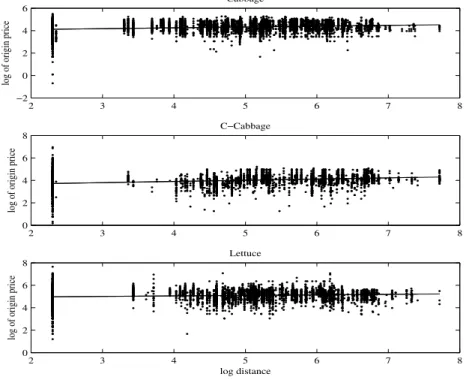
As mentioned, we use vegetable wholesale price data for Japan. In Japan, vegetables trade in a wholesale market in each prefecture, so we can obtain the price in the production prefecture (the origin price) and the price in the market (the market price). The origin price is used to measure quality, and from the market price information, the distance to market from the origin can be calculated. We depict the key observation in the relationship between quality and the distance to market using Figure 1. We plot the log of distance on the horizontal axis and the log of the origin price on the vertical axis. All figures illustrate a positive relationship between distance and origin price. Thus, there is a positive relationship in our data set.
Next, we report the results of the reduced-form regressions. As in the extant literature, we regress the price at the source on the distance to the destination:
lnpjj =const+ lnDnj+dumn+dumj+enj, (1) wherepjj is the price in regionj,const is a constant term,Dnj is the distance between originj and the market n,dumn is a market-specific term, dumj is a source-specific term, and enj is the error
2 3 4 5 6 7 8
−2 0 2 4 6
Cabbage
log of origin price
2 3 4 5 6 7 8
0 2 4 6 8
C−Cabbage
log of origin price
2 3 4 5 6 7 8
0 2 4 6 8
Lettuce
log distance
log of origin price
Figure 1: Logs of Distance and Source Price Relationship
term. Because we use the source price, pjj, where there is an interregional supply in the source prefecture j and a supply of the same product to market n from sourcej,pjj can act in a similar fashion to the FOB price in the literature. Using OLS, we find that there is a positive relationship between quality and distance, as reported in Table 2. Note that because Figure 1 illustrates the fitted value for the regression not controlling for region-specific effects, the positive relationship may result from regional shocks. However, we also estimate the regressions after including origin- and market-specific effects. The estimates reflecting regional-specific effects also display a positive relationship, as shown in Table 2.
Cabbage Cabbage C-cabbage C-cabbage Lettuce Lettuce
Distance 0.074 0.007 0.106 0.01 0.046 0.008
(0.002) (0.003) (0.03) (0.005) (0.003) 0.004
Num. of obs. 15841 15841 10803 10803 11565 11565
R-squared 0.065 0.494 0.105 0.504 0.019 0.364
Region-specific effect No Yes No Yes No Yes
Table 2: Origin Prices and the Distance Relationship
As discussed in the literature, several models can potentially explain this positive link. One of the possible candidates is quality sorting; that is, high-quality producers are able to supply
their goods to costly markets. Another is the presence of specific costs, which makes the relative price of high-quality goods lower in costly markets. Unfortunately, the results of the reduced- form regressions do not provide us with any information about the structural parameters, such as distance elasticity. Hence, the precise mechanism underpinning this empirical observation is unclear. The purpose of this analysis is then to identify the important structural parameters using quality heterogeneity models.
3. Model
We adopt a standard monopolistic competition, producer heterogeneity, product quality model following Baldwin and Harrigan (2011). An additional feature is the introduction of specific costs.
Assume there are N regions, and in each region, n, there is a continuum of producers whose mass is expressed by Mn.
A Cobb–Douglas constant elasticity of substitution (CES) utility function expresses the preferences of consumers in regionn:
Un= ( Z
ω∈Jn
(cnjqn)(σ−1)/σdω)(σ/(σ−1))µZ1−µ, (2)
whereJn is the set of products delivered to region n,cnj is the consumption of regionj’s goods in regionn,qn is the quality of these goods, andZ is the consumption of numeraire goods. Given the budget constraint,µYn=R
pnj(ω)cnj(ω)dω, the demand function is:
cnj(ω) = p−σnj q1−σn
Ynµ Pn1−σ
, (3)
wherePn= (R
(pnj/qn)1−σ)1/(1−σ) andYnis the income of the consumers in regionn. This signifies that as the quality of goods improves, consumer demand increases. Quality thus acts as a demand shifter in this setting.
We assume that producers produce a differentiated product, face local demandxnj(z), and maximize their profits. There is also a numeraire goods sector, in which a unit of goods is produced using a unit of labor. Thus, wage rates are set to one. On the cost side of the differentiated goods sector, producers must pay production and trade costs. The trade costs consist of ad valorem and specific costs. With regards to specific costs, we also assume that as in Irarrazabal et al. (2015), there is a perfectly competitive transport service sector. This service is available in every region, producers use t units of labor to supply goods of each unit, and thus producers have to incur additive trade costs tper unit of supply. We express the profits from market nusing:
πnj = (pnj−anjτnj−tnj)xnj−fnj, (4) where τnj is the ad valorem component, tnj is the specific component in trade costs, and ais the unit production cost.
Producers facing the local demand function (2) maximize their profits by setting the optimal price in market n:
pnj = σ
σ−1(τnjaj +tnj). (5)
Because we assume each producer makes a single product, we can replace the product indexωwith the producer’s productivity. This is the price of the good produced by a production costaproducer that consumers pay. We assume that there are no interregional trade costs for within-region trade such thatτjj= 0 and tjj = 1:
pjj = σaj
σ−1. (6)
Thus, by inverting the above price formula, we can express the cost level of the producer. Using this implied cost enables us to recover the quality level. In our data set, as we can observe the market price and the place of production, we can use the above relationship to identify the specific cost component separately from the ad valorem component.
We assume that product quality consists of two components: namely, observed and un- observed characteristics. A certain characteristic is related to quality (e.g., Crozet et al 2012;
Hummels and Schaur 2013). Because we consider that the sizes and grades of goods are observed and together capture some aspects of goods quality, the quality (qn) is a function of both observed and unobserved characteristics, qn =ξnjqnj, where ξnj is an observed factor (e.g., grade and size of goods) and qnj is unobserved. The latter quality factor, qnj, is assumed to be associated with production costs. Quality sorting implies that high-cost producers produce high-quality goods, and we thus assume a monotonic relationship between quality and production costs:
qnj=h(aj). (7)
This is required to estimate the quality-sorting model. If the relationship between costs and quality is not monotonic—for example, a U-shaped relationship—then we cannot identify the parameter that determines the quality-sorting pattern. We further assume a parametric form of h(.). As in Baldwin and Harrigan (2011), we suppose that the quality of products is a function of that cost level as follows:
h(aj) =a1+θj . (8)
Thus, if θ >−1, then high-cost producers produce high-quality goods. If θ >0 and specific costs are zero, then high-cost producers will deliver their products to more remote markets than low-cost producers because the rate of quality improvement exceeds the increase in cost. This provides the mechanism for quality sorting: high-cost producers produce high-quality goods, so they are more profitable than the goods of low-quality producers and accordingly can reach more costly markets.
If there are specific costs, then even if θ < 0, high-cost goods can also be highly profitable. We discuss this possibility in Sections 5.1 and 6.
We do not model quality as an endogenous choice, whereas in Kugler and Verhoogen (2012) and Lugovskyy and Skiba (2015), producers choose the quality level. Because our analysis employs data on agricultural products, the environment, which is exogenous to producers, largely determines the quality. Moreover, the resulting relationship from endogenous quality choice exhibits the same relationship between quality and production costs. Hence, we focus on empirically detecting the relationship between quality and cost.
With regard to trade costs, the key idea is that by using source and market prices, we can measure trade costs using price data. We normalize interregional trade costs by local trade costs incurred for local delivery. Thus, all trade costs are relative to the local cost of delivery. In addition, because price is a monotonic function of production costs, we can replicate costs using price data.
However, we assume a monotonic relationship between quality and production costs leading to the possibility of measuring quality using source price data. While quality can also be measured using explicit product characteristics (Crozet et al. (2012)), we derive the implied quality level using the source price information. As discussed in Section 2, this is mainly because there are unobservable quality characteristics.
The price differentials between markets and sources are:
pnj pjj
=τnj+ 1 aj
tnj. (9)
Hence, in the price differential equation, while we include the ad valorem term in the equation directly, the specific component is interacted with the cost term. This serves to identify the ad valorem and specific terms separately.2
The preceding price differential equation is observed only when there is actual delivery from j ton. Thus, we need to consider the producer’s delivery decision. The profit function is:
πnj = (σ−1σ )1−σ(τnjaj +tnj)1−σ q1−σn
Y µ
σPn1−σ −f. (10)
If profit is positive, there will be delivery from source j to market n. We construct a delivery decision variable, Vnj:
Vnj= [(σ−1σ )1−σ(τnjaj +tnj)1−σ q1−σn
Y µ σPn1−σ
]/f. (11)
IfV >1, then there is delivery from j ton. As Irarrazabal et al. (2015) show, because of specific costs, even the lowest-cost producer (a ≈ 0) earns finite profits. Thus, other than the above condition, there is a further selection condition, i.e., whether producer costs are sufficiently low
2In the extant literature, FOB prices measure quality. The role there is the same as in this analysis. However, there is a slight difference between the FOB and source price. By definition, the FOB price, pF OB, satisfies the following equation: pmarket=τ×pF OB+t.Thus,pF OB = (σ/(σ−1))(a+t/στ).However, because the source price is the price set for the source market without trade costs,psource= (σa/(σ−1)). Hence, while the source price does not depend on trade costs, it remains in the FOB price.
to obtain profits to cover fixed costs. We assume that this condition holds to focus on the entry condition.
To close the general equilibrium model, we assume that each consumer supplies one unit of labor for production, that there is a transport service sector using one unit of labor to ship one unit of goods, and that this service is freely used across regions as in Irarrazabal et al. (2015). This ensures that the wage rate is equal to one and there is a trade balance. However, to focus on the identification of trade costs, we simply analyze individual producer behavior. Regional fixed effects in the estimations capture the general equilibrium effects. For explicit treatment of the general equilibrium effects, we conduct Monte Carlo exercises to reveal how large trade cost reductions increase welfare in a later section.
4. Data
We conduct our empirical research using product-level data. We employ a daily data set of the wholesale prices of agricultural products in Japan known as the “Daily Wholesale Market Informa- tion of Fresh Vegetables and Fruits.”3 This daily market survey reports the wholesale prices and quantities sold of some 120 different fruits and vegetables. We use the 2007 report representing 274 market-open days.
The main advantage of this data set is that it includes information about individual product characteristics and detailed categorizations, such that we can classify each vegetable by brand, size, grade, and source region. For example, the cabbage category typically includes “cabbage,” “red cabbage,” and “spring cabbage.” For cabbage, our data set reveals that cabbages of size “6” and grade “syu” (excellent) were produced in Aichi Prefecture and traded in the Aichi and Tokyo markets on July 1, 2007, and that the prices of this type of cabbage were 31.5 yen per kg in Aichi and 36.8 yen per kg in Tokyo. Thus, we can calculate the price differential between these two locations, which we believe reflects the trade costs between the two prefectures.
Comparing the prices in different locations to infer trade costs is meaningful if the goods are identical and if the prices of these goods are comparable. As discussed, our data have a high degree of categorization, which is useful for the purpose of measuring trade costs. Furthermore, because our data represent information on agricultural products, goods can differ depending on the date of production. However, we do not have exact information on the production date, so we assume that these goods differ when trading dates differ. Because consumers may consider vegetables available on different dates differently, the information in our data set provides us with the identification of an identical product in terms of many product characteristics.
The price differential,pnj/pjj, that reflects trade costs is obtained by the difference between the wholesale price in the source prefecture j, pjj, and that in the consuming prefecture n, pnj.4
3Our data set is identical to that employed in Kano et al. (2013, 2014).
4All of the products are sold in markets, but not necessarily in their markets of origin. In this case, when we
The source price,pjj, is the price we observe for productωbeing delivered from the producer to the wholesale market in the source prefecture,j. If this product is also shipped to marketn, thenpnj is also observed. Thus, we setTnj = 1 for the pair (n, j) if we can calculate the price differentials, pnj/pjj.
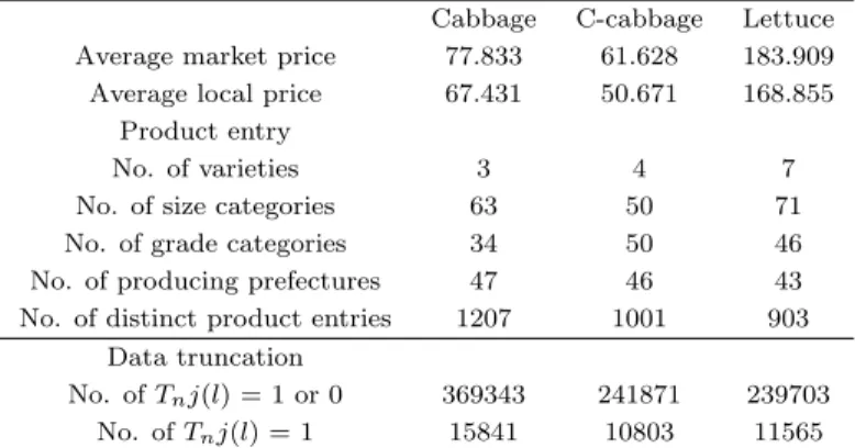
Cabbage C-cabbage Lettuce Average market price 77.833 61.628 183.909 Average local price 67.431 50.671 168.855
Product entry
No. of varieties 3 4 7
No. of size categories 63 50 71
No. of grade categories 34 50 46
No. of producing prefectures 47 46 43
No. of distinct product entries 1207 1001 903 Data truncation
No. ofTnj(l) = 1 or 0 369343 241871 239703 No. ofTnj(l) = 1 15841 10803 11565
Table 3: Summary Statistics
We focus our exercise on three vegetables; namely, cabbage, Chinese cabbage (c-cabbage, hereafter), and lettuce. As discussed in Section 2, these are vegetables priced higher in the source region and shipped to more distant markets. Table 2 summarizes several descriptive statistics for these products, indicating that each product is highly categorized by product variety, size, and grade. There are various kinds of measures of the grades and sizes; for grades, we have not only
“syu” (excellent) or “yu” (good), but also “A,” “B,” or “maru-syu” (good–excellent); for sizes, we have not only “L” or “M,” but also numeric “4,” “5,” or “2L”. The number of distinct product entries is thus quite large: 1,207 for cabbage, 1,001 for c-cabbage, and 903 for lettuce. Because the prices of vegetables with dissimilar characteristics are in fact different, even though vegetables might often be considered as a homogeneous good, in our case there is highly detailed product differentiation. This is consistent with the theoretical prediction by Antoniades (2015), in which there is a positive relationship between quality and price for heterogeneous products, but a negative correlation for homogeneous products. We also assume that these products differ when the trading date changes, so to a certain degree, our price differential data are the price differentials of identical products.
The average prices are 77.833 yen for cabbage, 61.628 for c-cabbage, and 183.909 for lettuce.
There are also market prices in the data. Because we use origin prices to measure quality, Table 2 also reports the prices at the origin. The average origin prices are 67.431, 50.671, and 168.855 yen for cabbage, c-cabbage, and lettuce, respectively. Thus, market prices outside the origin region
cannot observe both the market and source prices, we eliminate the product entry. If high-quality goods go to distant markets (i.e., prices increase by more in more distant markets than the increase in trade costs because of higher quality), then eliminating these observations may result in the under bias of the distance effect. Hence, our estimates serve as the lower bound of the distance effect.
are higher than those in the region. This is primarily because it is costly to ship goods to distant markets. Because trucks normally transport vegetables, and the truck transportation market in Japan is competitive, unlike Hummels et al. (2009), we do not need to consider markups in the transport sector. Our purpose is to address how much these price differentials reflect the shipping of high-quality goods to distant markets. Estimating a trade model to identify the key parameters should provide us with an answer to this question.
To understand the behavior of product shipment, we count the number of deliveryTnj(ω) = 1 and nondelivery Tnj(ω) = 0 cases. We identify product delivery Tnj(ω) = 1 if the data report that the source prefecture of product entryω sold in consuming regionnis regionj. If we observe no market price and only origin prices, then we set Tnj(ω) = 0. As shown in Table 1, there are some 230,000 delivery and nondelivery cases for each vegetable. This provides the number of observations for our full-information maximum likelihood (FIML) estimation. Out of the total number of delivery and nondelivery cases, the number of delivery cases (15,841, 10,803, and 11,565 for cabbage, c-cabbage, and lettuce, respectively) is relatively small. Our data set thus suggests that product delivery is limited. It is therefore clear that product delivery is local to the source prefecture. This raises some concerns with sample selection, and an additional concern about delivery patterns. If products do not ship to markets directly, then the actual delivery distance will be much longer than that between the final market and origin. This will cause over bias in the distance effects. However, the share of transferred vegetables is low, normally less than 7 percent according to the Ministry of Agriculture, Forestry and Fisheries.5 Thus, the influence of transit goods in our data is not significant.
As briefly mentioned in Section 2, we use the characteristic names to identify quality. A grade name including “syu” (excellent) means that the product is high quality. For example, the grade name, ‘maru-syu”, means ”good–excellent”, thus this is considered as high quality. Hence, if the grade characteristic name includes ”excellent”, then the high quality index takes a value of one and zero otherwise. Similarly, with regard to size, a size category including the letter “L” implies a large size. There are also other size categories such as ”S” (small), ”M” (medium), ”LL”, and
”L6”. We create an index variable such that the large size index takes a value of one if the size category name includes size ”L” and zero otherwise. The categorized shares of high-quality and large-size goods are substantial. For instance, for cabbage, 33.5 percent of goods are high quality and 49.5 percent are large size.
We also measure product quality with the origin price (the price in the source region). The reason is that even if the products share the same characteristics, consumers’ perceptions of quality may differ depending on unobservable factors or also on whether the product is available in the high or low season. For example, in the Tokyo market, the average price of cabbages of size “6”
and grade “syu” (excellent) produced in Aichi Prefecture is only 42.842 yen in January, but 86.638 yen in April. Thus, the source price, not the product characteristics, can capture the variation
5http://www.maff.go.jp/j/tokei/kouhyou/seika orosi/ (in Japanese).
in quality associated with the season in which traded. Because local shocks affect local market prices, we need to control for such specific effects. If demand shocks occur locally, the price will be higher without any improvement of quality. We consider this by including market-specific effects and monthly dummies in our estimations. When supply shocks take place (i.e., through an increase in production costs), the price will also be higher. If the cost associated with quality improvement increases, the Baldwin and Harrigan (2011) framework that we employ will capture it. Conversely, source-region-specific effects reflect cost shocks unrelated to quality.
With regard to the distance between regions, we define the inter-prefectural distance as the direct distance between prefectural head offices in the prefectural capital cities.6 We set the internal distance to 10 kilometers (km), which is shorter than the minimum inter-prefectural distance of 10.4 km (Kyoto–Shiga). We later use the Head and Mayer (2000) internal distance formula as a robustness check. Importantly, natural conditions, not just market conditions, may affect regional prices. For example, preferences and the production of vegetables may change according to the air temperature. We use daily temperature data for the market and the origin to control for these daily variations. As these are exogenous variables, they will also be helpful for identification of our selection models.
5. Empirical Specification
In this section, we specify the functional form of the transport cost functions and other elements for estimation. We assume that the ad valorem and specific components are a function of distance and other factors:
τnj =Dγnj1exp(const1+nj), (12) tnj=Dnjγ2exp(const2+nj), (13) whereconsti is the constant term and nj is the random component in trade costs.7
As we specify a monotonic relationship between price and production costs, we can invert this relationship in terms of price and insert it into the trade cost function. For simplicity, we assume that the remaining elements are common to the ad valorem and specific cost terms. Then, the log of the price differential equation is:
ln(pnj/pjj) =ln(Dnjγ1exp(const1) +1
aDnjγ2exp(const2)) +nj
= ln(Dγnj1exp(const1) +σ−1
pjjσ Dnjγ2exp(const2)) +nj. (14) Thus, using the variations ina(thereforepjj), we separately estimate γ1 and γ2.
6Available at http://www.gsi.go.jp/KOKUJYOHO/kenchokan.html
7As the minimum iceberg cost is one and the minimum specific cost is zero, the constant and unobservable terms are zero for iceberg costs and minus infinity for specific costs.
Because we do not observe factory (farmer) gate price in the data, we assume that the price differentials between the local price, pjj, and the unobservable farmer gate price, p0jj, are expressed in a similar way using local delivery costs, τ0j and t0j: pjj/p0jj = τ0j + (1/a)t0j. We additionally assume that the farmer gate price depends on a local price and random component, 0j: p0jj = pjjexp(0j). This enables us to investigate local delivery in an integrated fashion as the inter-prefectural trade case: pjj/p0jj = pjj/pjjexp(0j) = τ0j + (1/a)t0j ⇐⇒ ln(pjj/pjj) = 0 = ln(τ0j + (1/a)t0j) +0j. This treatment of intra-regional price differentials may cause a bias in the distance effect. While the true intra-regional price differentials are positive, treating these as zeros leads to overestimates. This is because the value of the dependent variable in the price differential equation is lower than its true value for small distance deliveries. Because ignoring local deliveries does not provide us an indication of the direction of biases, we deal with intra-regional price differentials in this form.
We estimate the parameter, θ, with the self-selection condition because qnj = a1+θ = (pjj(σ−1)/σ)1+θ:
lnV = ln( σ
σ−1)1−σ+ (1−σ) ln((pjj(σ−1)/σ)Dnjγ1exp(const1) +Dnjγ2exp(const2)) + (1−σ)nj
+ ln(Ynµ) + (σ−1) lnξnj+ (σ−1)((1 +θ)(lnpjj+ ln(σ−1)/σ)−lnσ−(1−σ) lnPn−fj, (15) where the fixed costs are assumed to consist of market and source fixed effects and a random com- ponent: fj = exp(λn+λj−fnj), as in Helpman et al. (2008). The observed product characteristics, including the indexes of high quality and large size, are incorporated in lnξnj. We estimate the system of these nonlinear equations (equation (14) and (15)) using FIML. The variables specific to each region, such as Yn or Pn, are controlled by prefecture-specific effects, and the fixed cost is decomposed into these regional-specific terms and a random component.
The source of selection bias is the fact that the error in the selection equation consists of the error from the price differential equation and other disturbances in the selection equa- tion. The conditional expectation of price differentials is expressed by: E[ln(pnj/pjj)|lnV ≥0] = E[ln(Dnjγ1exp(const1) + pσ−1
jjσDγnj2exp(const2))|lnV ≥ 0] +E[nj|lnV ≥ 0]. Because E[nj|lnV ≥ 0] =corr(, η)σσ
ηE[ηij|lnV ≥0] andηnj= (1−σ)nj+fnj, the error term in the price differential equation is correlated with that in the selection equation. Supposing that the delivery probability is expressed by P r = P r(lnV ≥ 0) and the predicted probability is ˆP r, then lnˆV = Φ( ˆP r)−1, where Φ is a standard normal distribution. We can express the bias term as an inverse Mills ratio:
E[ηnj|lnV ≥0] = E[ηnj|ηnj ≥ −lnˆV] =φ( ˆlnV)/Φ( ˆlnV), whereφ is the standard normal density (Helpman et al. (2008), Johnson (2012), Kano et al. (2013)). By construction and as a result of sample selection, these error terms are correlated, so we can capture the correlation by estimating the correlation parameterρ=corr(, η).
5.1. Distance elasticity of quality for the threshold producer
In the rest of this section, we discuss the interpretation of the estimating elasticity param- eters. As discussed earlier, empirical studies generally show that there is a positive relationship between the distance to market and the quality of goods, such that the model provides us with the signs of the elasticity of quality with respect to the distance to markets. For the purpose of discussion, let us begin by deriving the elasticity in the case of no specific costs for the threshold producer. From the zero-profit condition, the threshold value of cost,a∗, is expressed by:
(σ−1σ )1−σ(τnja∗)1−σ qn1−σ
Y µ
σPn1−σ −f = 0. (16)
By the implicit function theorem, we obtain the elasticity of costs with respect to distance from:
da∗Dnj
dDnja∗ = γ1
θ . (17)
Thus, the elasticity of threshold quality (q∗) with respect to distance is:
dq∗Dnj
dDnjq∗ = (1 +θ)γ1
θ . (18)
If trade cost is an increasing function of distance (γ1 >0) and the speed of quality improvement is relatively high (θ >0), then this elasticity is positive.
In the presence of a specific type cost, the zero-profit condition is:
(σ−1σ )1−σ(τnja∗+tnj)1−σ qn1−σ
Ynµ σPn1−σ
−f = 0. (19)
Similarly, by the implicit function theorem, the elasticity is:
da∗Dnj
dDnja∗ = γ1Dγ1e1 +γ2Dγ2e2a∗−1
θDγ1e1+ (1 +θ)Dγ2e2a∗−1. (20) The sign of the above elasticity depends on not only γ1 and θ, but alsoγ2 and 1 +θ. As long as γ2 >0 and θ > −1, the elasticity will be positive, even if θ < 0. Thus, observations of a positive link between quality and distance do not necessarily imply a high degree of quality improvement.
Indeed, even if the quality improvement rate is low, the demand force captured by the presence of specific costs may account for the positive relationship. The presence of specific costs relaxes the condition that quality improvements create a positive link between quality and the distance to market.
We can illustrate this quality-sorting mechanism using the thresholds for distance, not productivity. Let us define the zero-profit distance, D∗, given the productivity, a:
(D∗γ1a+D∗γ2)a−(1+θ)= (σ/(σ−1))−1(σP1−σf /µY)1/(1−σ).
If t = 0, the above condition turns out to be: D∗ =aθ/γ1(σ/(σ−1))−1/γ1(σP1−σf /µY)1/(1−σ)γ1. Hence, if θ > 0 andγ1 > 0, then the higher the cost (a largea) is, and the longer the zero-profit distance (largeD∗) is. Ift6= 0, then we obtain:
dD∗/da=−a−θ−1((−θ)D∗γ1 −(1 +θ)D∗γ2a−1)/(γ1D∗γ1−1a1−θ+γ2D∗γ2−1a−(1+θ).
The denominator of this expression is positive. So, if the numerator is positive, then the higherais, the higher D∗ is. This is true even ifθ <0 as long as the second term in the numerator dominates the first term. Therefore, it is profitable to supply high-quality products to distant markets, even if the quality improvement rate is low.
6 Illustration of Bias
Before conducting the empirical analysis using actual data, we illustrate how trade cost data appear depending on the data-generating processes. We create a linear economy geographically sequentially separated into 47 regions on the integer line between 1 and 47. This linear economy implies that the distance between regions iand j,dij, is equal to |j−i|with a minimum distance of 1 and a maximum distance of 46.
To understand the idea behind the positive and negative relationships between the quality of goods and the distance to markets, we generate the data using the model of both quality and specific costs from the previous section and an only-quality model for a positive or negative quality cost parameter (θ). We draw 4,700 (= 100×47 prefectures) sets of Gaussian random variables for the fixed and trade cost components,fij and ij, respectively, independently of their distributions.
The elasticities of trade costs with respect to distance are set to 0.5 for the ad valorem and specific costs. The top panel of Figure 2 depicts the relationship between quality and distance when theta is positive (θ= 0.5). As shown, both models create a positive relationship: the slope of the only- quality model is 0.236, and that of the model with quality and specific costs is 0.315. The middle panel plots the relationship between distance and quality for a large negative theta (θ = −0.5).
Both figures reveal a negative correlation: the slope of the only-quality model is -0.073, and that of the quality and specific costs model is -0.008. Thus, low-quality (low-cost) products ship to long-distance markets.
The most notable relationship is revealed in the bottom panel of Figure 2, which is generated under a moderately negative theta (θ = −0.15). The left-hand-side figure is the model with quality and specific costs and reveals a positive relationship (the slope is 0.216). In contrast, the right-hand-side figure is the only-quality model and depicts a negative relationship (the slope is - 0.045). Hence, we observe a positive relationship between quality and distance when the underlining data-generating process is from the model of quality and specific costs, even though the quality improvement rate is not high. In this sense, the positive relationship between quality and distance may result from either a strong (θ > 0) or moderate (θ = −0.15) quality improvement and the presence of specific costs.
To explicitly demonstrate the estimation biases when there is a moderate quality improve- ment (θ =−0.15) and specific trade costs, we conduct Monte Carlo experiments using the model from the previous section to show that the estimates using a model without specific costs account for the bias. We first generate artificial data using the model with both quality and specific costs.
Figure 2: Quality and Distance to Market Relationship under Different θs
We then estimate the model without specific costs, followed by an estimation using the true model with quality and specific costs. We assume that the shape of the demand function is common across the regions and characterized by an elasticity of substitution parameter of 3.75. Because we focus on estimates using a model with regional fixed effects, we characterize each region with aggregate price and aggregate real expenditure, both of which we set to 20.00. For simplicity, we ignore the cross-regional variations in productivity. We assume that in each region, a product is produced with a productivity level equal to 0.99 and a factor cost set to one. Gaussian random components appear in both the fixed and trade costs. In the fixed costs, the random term has a standard deviation of 0.65. Idiosyncratic random variations in trade costs are captured by a standard deviation of 0.25.
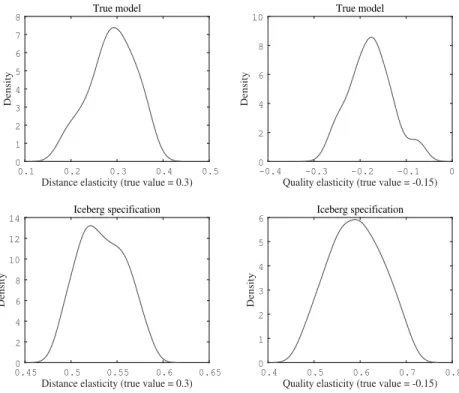
To validate the Monte Carlo experiment, we again draw 4,700 sets of fij and ij and then calculate the price differentials and the selection equation under the hypothesized value of the distance elasticity of trade costs, being 0.3 for the ad valorem trade cost and 0.5 for the specific trade cost. In each Monte Carlo draw of the true value of the distance elasticity, we implement our estimations of the distance elasticity. The first is the FIML estimation without specific costs (an iceberg-type specification), and the second is the FIML with specific costs. By construction, the FIML estimation without specific costs suffers misspecification bias. Because the ad valorem component captures the trade cost associated with the specific component, there will be over
bias in the distance elasticity of the ad valorem trade costs. Similarly, because the presence of specific costs delivers high-quality goods to distant markets, the elasticity of quality with respect to costs also captures this effect. If this quality elasticity is high, high-quality products are highly profitable, and thus shipped to distant markets. With specific costs, the distance elasticity of specific costs correctly estimates this Alchian–Allen effect. However, without specific costs, the positive relationship between quality and the distance to market will be included in the quality elasticity estimates.
Figure 3 depicts the non-parametrically smoothed densities of the distance and quality elasticity estimates with the Gaussian kernel. The top panel corresponds to the model with specific costs and the bottom panel to that without. The figures in the top panel show that the estimates using the true model are consistent and distributed around the underlying true value: the median value of γ1 is 0.277 and that of θ is -0.171. However, the figures in the bottom panel reveal that the estimates using the model without specific costs are subject to severe over bias. As we have argued, while the true ad valorem distance elasticity is 0.3, the median value of the estimates is 0.536. Similarly, while the true quality elasticity is -0.15, the median is 0.591. We calculate the Bayesian Information Criterion (BIC) to evaluate the performance of the models. All BIC values under the true model estimations are lower than the values under the model with quality only, which suggests that the true model fits the data better than the quality-only model. Hence, the Monte Carlo exercise confirms the necessity of incorporating a specific cost component for drawing correct inferences on the distance and quality elasticities.
To allow for the situation where the quality-only model—and not the quality-specific cost model—generates the real data, we now consider the case where the quality-only model is the true model. Accordingly, we conduct a simulation where the data are generated by the model with only quality and then estimate it using the quality-only and quality-specific cost models. If the true data-generating process is from the quality-only model, there will be misspecification in the model with quality and specific costs, and we would wrongly attribute the distance relationship to the specific cost factor. To address this, we again calculate BIC under the quality-only model estimations (in our exercise, this is the true model) and under the model with quality and specific costs. We find that BIC under the quality-only model is lower than under the quality-specific cost model for 89 percent of the Monte Carlo trials. Moreover, the distance elasticity of specific cost has the wrong sign (it is negative). Accordingly, we are able to reveal if a model generates quality-only real data using BIC calculations and by checking the signs of the estimated parameters.
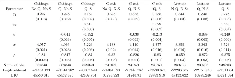
7. Results: Relationship between Quality and Distance
In this section, we report our estimation results. To demonstrate the importance of incor- porating both goods quality and specific costs, we conduct our estimations using several different specifications: 1) structural estimation of a simple Melitz (2003) model, 2) structural estimation
Distance elasticity (true value = 0.3)
0.1 0.2 0.3 0.4 0.5
Density
0 1 2 3 4 5 6 7
8 True model
Quality elasticity (true value = -0.15)
-0.4 -0.3 -0.2 -0.1 0
Density
0 2 4 6 8
10 True model
Distance elasticity (true value = 0.3)
0.45 0.5 0.55 0.6 0.65
Density
0 2 4 6 8 10 12
14 Iceberg specification
Quality elasticity (true value = -0.15)
0.4 0.5 0.6 0.7 0.8
Density
0 1 2 3 4 5
6 Iceberg specification
Figure 3: Kernel Densities of Estimators of Distance and Quality Elasticities
with a quality model (as in Baldwin and Harrigan (2011)), and 3) structural estimation of a firm- heterogeneity model with quality and specific costs. To compare the results with those in the extant literature, we begin by specifying no quality dimension and no specific costs.
Columns 1, 4, and 7 in Table 3 provide the results of a model without a quality dimension for cabbage, c-cabbage, and lettuce, respectively. The important parameters are the elasticity of substitution and the elasticity of transport cost with respect to distance. The substitution parameters are 4.957, 4.138, and 3.355 for cabbage, c-cabbage, and lettuce, respectively. These values are reasonable in the context of studies of individual product data. The distance elasticity parameters are 0.227, 0.325, and 0.343 for cabbage, c-cabbage, and lettuce, respectively. These are similar to the results in Kano et al. (2013). Thus, the distance effect is larger than that in the literature using price data (Engel and Rogers (1996), Parsley and Wei (1996, 2001), Crucini et al.
(2010, 2015), and Atkin and Donaldson (2015)), and this may be because, unlike here, there is no controlling of the sample selection problem.
We now introduce quality, as in Baldwin and Harrigan (2011). The results are in Columns 2, 5, and 8 in Table 3. As shown, the estimates of the distance effect (0.228, 0.325, and 0.345 for cabbage, c-cabbage, and lettuce, respectively) and the elasticity of substitution (4.966, 4.149, and 3.363 for cabbage, c-cabbage, and lettuce, respectively) are almost identical to those without quality. The quality parameters turn out to be marginally negative, which suggests that high-cost