Relation between Z 3 symmetry and sign problem

(1)

九州大学学術情報リポジトリ

Kyushu University Institutional Repository

Z3対称性と符号問題の関係とグラディエントフローに基づく純SU(2)ゲージ理論の解析

開田, 丈寛

https://doi.org/10.15017/4059986

出版情報：Kyushu University, 2019, 博士（理学）, 課程博士バージョン：

権利関係：

(2)

Relation between Z ³ symmetry and sign problem

and

analyses of pure SU(2) gauge theory based on gradient flow

Takehiro Hirakida

Theoretical Nuclear Physics, Department of Physics

Graduate School of Science, Kyushu University

744, Motooka, Nishi-ku, Fukuoka 819-0395, Japan

(3)

(4)

Abstract

Quantum chromodynamics (QCD) describes the dynamics of quarks and gluons, and the QCD states depend on temperature and the quark chemical potential. In the low temperature and the small quark chemical potential region, quarks are confined in hadrons. In the high temperature region, quarks and gluons are in the quark-gluon plasma phase. In the low temperature and the large quark chemical potential region, it is considered that there is the color superconductor phase.

One of methods to investigate QCD states is lattice QCD. By using the theory, we can treat non-perturbative properties of QCD, and in fact many calculations have been made in both the zero and the finite temperature regions. On the other hand, in the finite quark chemical potential region, it is too diﬃcult to obtain reliable results due to a numerical problem called the sign problem. In this thesis, in order to investigate properties of QCD in the finite quark chemical potential region, we focus on two approaches:

Z3-QCD and 2-color QCD.

1. Z3 symmetry and sign problem

The QCD-like model with exact Z3 symmetry is called Z3-QCD. It is known that Z3-QCD agrees with the ordinary QCD in the zero temperature limit, and numerical simulations with the spin model indicate that the sign problem of Z3-QCD becomes much milder than QCD.

Thus, investigatingZ3-QCD gives hints for QCD properties in the zero temperature and the finite quark chemical potential region. In this thesis, we use the effective Polyakov-line model as an effective model of lattice QCD, and discuss the relation betweenZ3 symmetry and the sign problem. The numerical results by using the reweighting method show that the region where the sign problem occurs is narrower in the Z3 symmetric model than that in the model corresponding to the ordinary QCD. We also improve the reweighting method, and this makes the sign problem less serious in the effective model.

2. Analyses of pure SU(2) gauge theory

The sign problem is absent in 2-color QCD, so that it is possible to make numerical calculations in the finite quark chemical potential region. Therefore, we can check the validity of eﬀective models by comparing both model and lattice results. When constructing an eﬀective

i

(5)

ii

model, we need thermodynamic quantities of pure SU(2) and SU(3) gauge theories. The thermodynamic quantities also have an important role to know properties of both 2-color and 3-color QCD. Recently, the gradient flow method to measure the thermodynamic quantities via the energy-momentum tensor was developed. In this thesis, we use this method to study the thermodynamics for pure SU(2) gauge theory.

We determine the scale-setting function precisely, and measure thermodynamic quantities through the energy-momentum tensor. Our results are consistent with data obtained by the other methods in the high temperature region. By comparing our results with the results of pure SU(N_c ≥ 3) gauge theory, we confirm that our results have diﬀerent behavior due to the diﬀerence of the order of the phase transition.

This thesis is based on the following published papers:

• Sign problem in aZ₃-symmetric eﬀective Polyakov-line model T. Hirakida, J. Sugano, H. Kouno, J. Takahashi, and M. Yahiro, Phys. Rev. D 96, 074031 (2017).

• Thermodynamics for pure SU(2) gauge theory using gradient flow T. Hirakida, E. Itou, and H. Kouno,

Prog. Theor. Exp. Phys. 2019, 033B01.

(6)

List of Figures

1.1 Energy-scale dependence of the running coupling constant α_s . 2

1.2 QCD phase diagram . . . 5

2.1 Conceptional diagram of the FTBC . . . 11

2.2 Allowed region ofP_x and Q_x . . . 15

2.3 Re[L_F] in theφ_r,x–φ_g,x plane . . . 16

2.4 Re[L_F,Z₃] in the φ_r,x–φ_g,x plane . . . 17

2.5 Eﬀective potentialL_H from the Haar measure inφ_r,x–φ_g,x plane. 18 2.6 µ/M-dependence of ∆L_F,R . . . 19

2.7 Re[L_F]–Im[L_F] or Re[L_F,_Z₃]–Im[L_F,_Z₃] relation in the case of N_f = 3 . . . 20

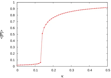
2.8 κ-dependence of ⟨|P¯|⟩ at µ= 0 . . . 22

2.9 Scatter plot ofP_x . . . 22

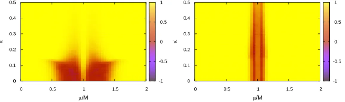
2.10 κ- and µ-dependence of the reweighting factor for EPLMWO and Z3-EPLM . . . 23

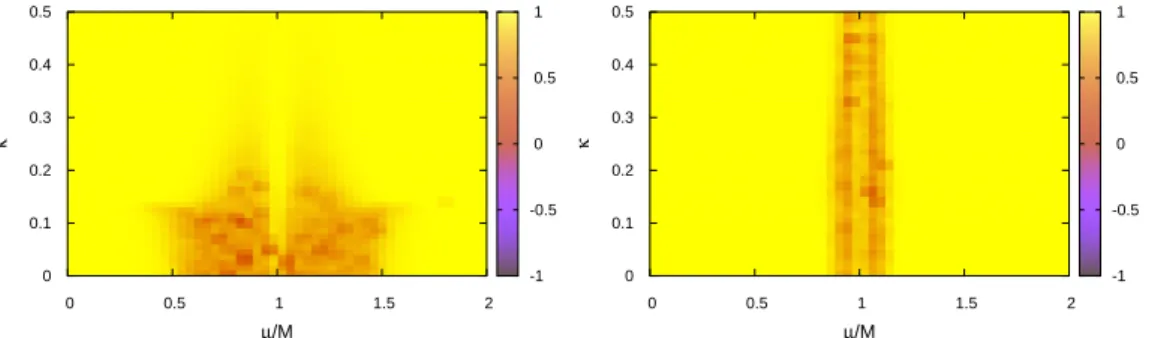
2.11 κ- andµ-dependence of the ration W^′′/W˜^′′ for EPLMWO and Z3-EPLM . . . 24

2.12 µ- andNs-dependence of the reweighting factors in EPLMWO and Z3-EPLM with both PQRW and IPQRW . . . 25

2.13 µ- and Ns-dependence of ⟨|P¯|⟩ in EPLMWO and Z3-EPLM with both PQRW and IPQRW . . . 26

2.14 µ- andN_s-dependence ofn_q in EPLMWO andZ3-EPLM with both PQRW and IPQRW . . . 27

2.15 µ-dependence ofW^′ and n_q in EPLMWO and Z3-EPLM with M/T = 30 at κ= 0.0 . . . 28

3.1 Comparison oft²⟨E(t)⟩between the lattice result and the perturbative calculation . . . 35

3.2 t/a²-dependence of t²⟨E(t)⟩ with both plaquette and clover- leaf definitions . . . 36

3.3 Ratio of the lattice spacing log(a²/a²₀) . . . 37

3.4 Continuum extrapolation of ratios of √ 8t₀ and r₀ orr_c . . . . 38

3.5 Continuum extrapolated 8t₀σ . . . 39

3.6 Flow time dependence of ∆/T⁴ and s/T³ . . . 41

3.7 Extrapolation ofa→0 . . . 42 v

(9)

vi LIST OF FIGURES 3.8 Extrapolation oft→0 . . . 43 3.9 Results of the entropy density, trace anomaly, and equation of

state . . . 44 3.10 Comparison with the prediction of the Hard-Thermal-Loop

model . . . 45 3.11 N_c-dependence of the rescaled trace anomaly (∆/T⁴)/(P_SB/T⁴) 46 A.1 Topological charge for 600 configurations at β = 2.85 . . . 52

(10)

List of Tables

3.1 Simulation setup for the scale setting and the results of t₀/a² . 37

3.2 Parameter sets for the finite temperature simulation . . . 40

3.3 Results of thermodynamic quantities . . . 44

A.1 Results of t0/a² for severalA. . . 52

A.2 Ratios a/a₀ for severalA . . . 53

A.3 Coeﬃcients of the scale-setting functions for several A. . . 53

vii

(11)

(12)

Chapter 1 Introduction

1.1 Quantum chromodynamics

The interaction between quarks and gluons is called strong interaction, one of the four fundamental interactions. The theory describing this interaction is quantum chromodynamics (QCD). This theory is non-Abelian gauge theory with the color SU(3) group. The Lagrangian density of QCD in Euclidean spacetime is written by

LQCD= ¯q(γ_µD_µ+M)q+ 1

2g²tr_c[F_µνF_µν], (1.1)

Dµ=∂µ+iAµ, (1.2)

F_µν =∂_µA_ν−∂_νA_µ−i[A_µ, A_ν] =−i[D_µ, D_ν], (1.3) where q, ¯q, and A_µ are quark, antiquark, and gluon fields, M is the quark mass, and g is the coupling constant. In Eq. (1.1), tr_c denotes the trace of color indices. With the SU(3) generatorT^a, gluon fields are written by A_µ=

∑

aA^a_µT^a. The Lagrangian density LQCD is invariant under the following local gauge transformation:

q(x)→V(x)q(x), q(x)¯ →q(x)V¯ ^†(x), (1.4) Aµ(x)→V(x)Aµ(x)V^†(x) +i(∂µV(x))V^†(x), (1.5) where V(x) = exp [iθâ(x)Tâ] with real parametersθâ.

So far, six quarks have been discovered: up (u, m_u ∼ 2.3 MeV), down (d, m_d ∼ 4.8 MeV), strange (s, m_s ∼ 95 MeV), charm (c ,m_c ∼ 1.3 GeV), top (t, mt ∼173 GeV), and bottom (b, mb ∼ 4.2 GeV). The typical energy scale of QCD is Λ_QCD∼200 MeV. Therefore, quarks with lighter mass than Λ_QCD have been discussed for many years.

One of the most important properties of QCD is the asymptotic freedom.

This property comes from the fact that the eﬀective coupling constant (the running coupling α_s) becomes small in the high energy scale or at the short distance. However, the coupling gets large in the low energy scale or at the long distance. The running coupling α_s as a function of the energy scale Q

1

(13)

2 CHAPTER 1. INTRODUCTION is shown in Fig. 1.1. The perturbative theory reproduces the experimental results at the high energy scale where α_s < 1. In the low energy scale, however, the perturbative analysis is unsuitable due to the large running coupling, and the non-perturbative features appear, e.g. the spontaneous breaking of chiral symmetry and the quark confinement.

Figure 1.1: Energy-scale dependence of the running coupling constantα_s[1].

1.1.1 Spontaneous breaking of chiral symmetry

For simplicity, let us consider the quark part of 2-flavor QCD,

Lq = ¯q(γµDµ+ ˆM)q, (1.6) where q = (u, d)^t, ˆM = diag(mu, md). By using the chirarity operator γ5 ≡ γ₁γ₂γ₃γ₄, we can divide quark fieldsq into

q =q_R+q_L, q_R,L=P_R,Lq, P_R= 1

2(1 +γ₅), P_L= 1

2(1−γ₅). (1.7) Then, the quark part of the Lagrangian densityLq becomes

Lq = ¯q_Rγ_µD_µq_R+ ¯q_Lγ_µD_µq_L+ ¯q_RM q_L+ ¯q_LM q_R. (1.8)

(14)

1.1. QUANTUM CHROMODYNAMICS 3 In the massless limit M = 0, the Lagrangian density is invariant under the U(2)_R⊗U(2)_L transformation

q_R,L→V(θ)_R,Lq_R,L, V(θ) = exp [

i

∑3 a=0

θ^a_R,LT^a ]

, (1.9)

whereT⁰ is the 2×2 unit matrix and Tⁱ (i= 1,2,3) is the SU(2) generator.

This symmetry is called chiral symmetry. The transformation (1.9) is rewrit- ten into U(1)_V⊗U(1)_A⊗SU(2)_V⊗SU(2)_A. The U(1)_Asymmetry is broken by the chiral anomaly, and the symmetry is broken into U(1)_V⊗SU(2)_V due to the spontaneous symmetry breaking.

The order parameter of the spontaneous breaking of chiral symmetry is the quark condensation ⟨qq¯⟩: ⟨qq¯⟩ = 0 when chiral symmetry is preserved, and ⟨qq¯⟩ ̸= 0 when the symmetry is broken spontaneously. When the symmetry is broken spontaneously, n massless bosons (NG-bosons) are generated, where n is the number of generators for the broken symmetry (Nambu-Goldstone theorem). In the case of 2-flavor QCD, the generated massless bosons are three pions (π⁰, π^±).

In 2-flavor QCD, quarks have finite but small masses. Therefore, chiral symmetry is approximately preserved, and hence NG-bosons have small masses. In the spontaneous chiral symmetry broken phase, the quark condensation ⟨qq¯⟩ is finite, so that the nucleon masses become larger than the sum of masses of three quarks.

1.1.2 Quark confinement

The interaction between a quark and an antiquark becomes larger as the running coupling αs increases. Thus, when αs is large, quarks are confined in hadrons and we cannot observe quarks alone. This property is called the quark confinement, and the transition into the deconfined state is called the confinement-deconfinement transition. This transition is related to the center symmetry of QCD (Z3 symmetry).

In QCD, we usually take the boundary conditions for quark and gluon fields in the temporal direction as

q(x, x4 = 1/T) =−q(x, x4 = 0), (1.10) A_µ(x, x₄ = 1/T) =A_µ(x, x₄ = 0). (1.11) For the gauge transformation V(x), we take the boundary condition as

V(x, x₄ = 1/T) =V(x, x₄ = 0). (1.12) Under the gauge transformation with Eq. (1.12), the Lagrangian density (1.1) and the boundary conditions (1.10) and (1.11) are not changed. Next,

(15)

4 CHAPTER 1. INTRODUCTION we consider the gauge transformation with the Z3 transformed boundary condition:

V(x, x₄ = 1/T) = e⁻^i2πk/3V(x, x₄ = 0) (k ∈Z). (1.13) By using this, the boundary condition for quark fields (1.10) is changed into q(x, x₄ = 1/T) =−e^i2πk/3q(x, x₄ = 0), (1.14) while that for gluon fields (1.11) is invariant. Therefore, Z3 symmetry of QCD with quarks is explicitly broken via the boundary condition (1.10).

Now, let us consider pure SU(3) gauge theory at finite temperature.

Gluon fields Aµ(x) are periodic in the temporal direction, and we can construct the following gauge-invariant operator,

L(x)≡ 1

N_cT exp [

i

∫ 1/T 0

dx₄ A_µ(x, x₄) ]

, (1.15)

where T denotes the time-ordered product, and N_c represents the number of colors. This is called the Polyakov loop. Under the gauge transformation with the boundary condition (1.13), this operator is changed into

Φ(x)≡tr_c[L(x)]→e⁻^i2πk/3Φ(x). (1.16) It is known that the confinement-deconfinement transition is the first order, and ⟨Φ⟩ is finite at high temperature and zero at low temperature. This quantity breaksZ3 symmetry, so ⟨Φ⟩ is an order parameter of it.

In the infinite quark mass limit, ⟨Φ(x)⟩ is derived by

⟨Φ(x)⟩=e⁻^F^q^/T, (1.17) whereF_qis the free energy of the static quark. When⟨Φ(x)⟩= 0,F_qdiverges.

This indicates that we need the infinite energy to obtain a quark, and thus quarks are confined in hadrons. On the other hand, whenF_q is finite,⟨Φ(x)⟩ is also finite, and then we can extract a quark.

1.1.3 Phase diagram of QCD

The states of quarks and gluons depend on temperature T and the quark chemical potentialµ_q. In the lowT and the lowµ_q region, quarks are confined in hadrons, and this phase is called the hadronic phase, where Z3 symmetry is weakly preserved and chiral one is weakly broken. In the high T region, quarks and gluons are in the quark-gluon plasma (QGP) phase, where they behave almost as free particles. In this phase, Z3 symmetry is broken and chiral symmetry is restored. In the low T and the large µq region, it is considered that there is the color superconductor phase, where the cooper

(16)

1.2. LATTICE QCD 5 pairs of quarks are formed. This phase is expected to exist inside of the high density star such as a neutron star.

The schematic figure, so-called the QCD phase diagram, is shown in Fig. 1.2. This diagram is investigated by both theoretical and experimental studies, but the wide region, i.e. the finite µ_q region, is not understood com- pletely. Thus, investigating the QCD phase diagram in the finite µ_q region is one of the most important subjects in hadron physics.

Figure 1.2: QCD phase diagram in the µ_B–T plane [2], where µ_B is the baryon chemical potential (µ_B = 3µ_q).

1.2 Lattice QCD

The lattice QCD (LQCD) simulation is one of methods to study the QCD phase diagram. LQCD is formulated in the discretized spacetime, and the partition function after integrating quark fields is given by

Z =

∫

DU det[M(µ_q)] exp [−S_G], (1.18) S_G =

∫

d⁴x 1

2g²tr_c[F_µνF_µν], (1.19) M(µq) =γµDµ+m−γ4µq, (1.20) where det[M(µq)] is the fermion determinant, and U is the link variable defined by

U_µ(x) = exp [iaA_µ(x)], (1.21) where a is a lattice spacing.

(17)

6 CHAPTER 1. INTRODUCTION In LQCD simulations, the Monte Carlo method is usually used to evaluate the integration in the partition function (1.18). Then, we treat the integrand ρ(µ_q) = det[M(µ_q)]e⁻^S^G as a probability weight, so that ρ(µ_q) is needed to be real and positive.

1.2.1 Sign problem

The determinant det [M(µ_q)] satisfies the following relation:

(det [M(µ_q)])^∗ = det[

γ₅M(−µ^∗_q)γ₅]

= det[

M(−µ^∗_q)]

. (1.22)

When µq is zero or a pure imaginary number, the determinant becomes real.

However, when µ_q is real or complex, the determinant becomes complex.

Therefore, LQCD simulations based on the Monte Carlo method are much diﬃcult. This problem is so-called the sign problem.

To avoid the sign problem, several methods are proposed and tested, e.g.

the reweighting method [3], and the Taylor expansion method [4, 5]. Recent years, numerical simulations based on the Complex Langevin method [6–8]

and the Lefschetz thimble method [9, 10] have progressed. However, it is still too diﬃcult to obtain reliable results especially in the large µ_q region.

1.2.2 Z

³

-symmetric QCD-like model and sign problem

As mentioned in Sec. 1.1.2, Z3 symmetry in QCD with dynamical quarks breaks explicitly through the boundary condition for quark fields. For the three flavor case, instead of the ordinary boundary condition for quarks, we can restoreZ3 symmetry by introducing the flavor-dependent twist boundary condition [11]. The QCD-like model with this condition is called Z3-QCD, and its properties were investigated by using an eﬀective model such as the Polyakov-loop-extended Nambu–Jona-Lasinio (PNJL) model [11–15]. In addition, the lattice simulation of Z3-QCD was carried out at µ_q = 0 [16], and the results were consistent with the PNJL-model predictions.

In Ref. [15], it was also predicted that the sign problem becomes milder in Z3-QCD than in the ordinary QCD. In order to examine this prediction, Hirakida et al. [17] performed a numerical simulation by using the Z3-symmetric 3D several-state Potts model as a toy model of Z3-QCD. It was confirmed that the sign problem is much milder in the Z3-symmetric model than in the model without exact Z3 symmetry. Thus, it is expected that we can perform the lattice calculation of Z3-QCD in the large quark chemical potential region.

(18)

1.2. LATTICE QCD 7

1.2.3 Sign problem in 2-color QCD

In 2-color QCD, the fermion determinant satisfies the same relation shown in Eq. (1.22). In addition, the determinant also has the following relation:

det[M(µ_q)] = det[(σ₂Cγ₅)^†M(µ_q)(σ₂Cγ₅)] = det[M(µ^∗_q)]^∗, (1.23) whereC ≡γ₂γ₄ is the charge conjugation matrix, andσ₂ is the second Pauli matrix in the color space. Due to this relation, the fermion determinant becomes real, and it is possible to carry out lattice calculations of 2-color QCD in the real µ_q region. In fact, several calculations were done in Refs.

[18–29].

Once obtaining thermodynamic quantities and the expectation value of the Polyakov loop of pure SU(2) gauge theory, it is possible to construct an eﬀective model of 2-color QCD. In Refs. [27, 30, 31], the PNJL model for 2-color QCD was constructed and the validity of the model was tested by comparing the model and the lattice results. However, in these researches, thermodynamic quantities of pure SU(2) gauge theory are not used to determine the eﬀective potential. Thus, these model results may not be realistic.

It is needed to improve the eﬀective Polyakov loop potential by using lattice results of pure SU(2) gauge theory.

1.2.4 Thermodynamic quantity of pure SU(N

_c

) gauge theory

Thermodynamic quantities have an important role to know properties of QCD. Several methods (e.g. integral method [32], moving-frame method [33]) have been proposed and used in lattice calculations of both pure SU(N_c) gauge theory and QCD with dynamical quarks. These results in pure SU(Nc) gauge theory are consistent with the prediction of the gluon gas model and the Hard-Thermal-Loop model [34] in the high temperature region, while they are well explained by the massive glueball model in the low temperature region.

Transport coeﬃcients are also important in the finite temperature region.

For intermediate temperature, experimental data show the small ratio of the shear viscosity to the entropy density η/s. This result indicates that the QCD state in that temperature is consistent with a perfect liquid rather than a gas [35]. In the theoretical side, the work in Ref. [36] shows the lower bound for η/s by using a large-N_c analysis based on AdS/CFT correspon- dence. However, the correction terms of 1/N_c have not been determined yet. In lattice calculations, methods to obtain viscosities were proposed and tested [37–40]. The first step is measuring the correlation function of the energy-momentum tensor (EMT), and there are several problems, e.g. the small signal-to-noise ratio of correlation functions [39], the definition of the

(19)

8 CHAPTER 1. INTRODUCTION renormalization of the EMT as a conserved quantity on the lattice, and obtaining the spectral function from correlation functions.

In the lattice gauge theory, constructing the EMT on the lattice is also diﬃcult, since the lattice regularization breaks the translational symmetry.

In recent years, Suzuki proposed a new method to measure the EMT in Ref. [41] by using the gradient flow [42, 43]. When using this method, the statistical error becomes smaller than that by the other methods, and the wave function renormalization of the EMT is not needed in pure SU(Nc) gauge theory. Due to these advantages, the method based on the gradient flow was applied to pure SU(3) gauge theory [44], and the result is consistent with that obtained by other methods. Moreover, this method has been extended to QCD with dynamical quarks [45]. Therefore, by applying this method, it is expected that the results of pure SU(2) gauge theory provide the large signal for the 1/Nc correction terms.

1.3 Strategy

It is important to investigate the QCD phase diagram at the finite quark chemical potentialµ_q. One of methods to study the QCD dynamics is LQCD simulations. However, it is diﬃcult to carry out LQCD simulations at the finite quark chemical potential due to the sign problem. In order to avoid this problem, several applications are proposed, but it is still diﬃcult to obtain reliable results. In this thesis, we adopt two approaches to investigate properties of QCD in the real µ_q region: Z3-QCD and 2-color QCD.

Z3-QCD agrees with the ordinary QCD in the zero temperature limit.

In Ref. [17], the numerical simulation with the spin model as the QCD-like model shows that the sign problem is much milder in theZ3symmetric model than in the QCD-like spin model. Therefore, it is expected that the approach with Z3-QCD gives hints for properties of QCD in the zero temperature and the finiteµ_qregion, e.g. nuclear matters and neutron stars. In this thesis, we use the effective Polyakov-line model [46] as an effective model of LQCD, and make numerical simulations based on the reweighting method in the finiteµ_q region. We also improve the reweighting method and test the efficiency of it with the effective Polyakov-line model.

In lattice calculations of 2-color QCD, there is no sign problem since the fermion determinant becomes real. Therefore, we can check the validity of effective models such as the PNJL model by comparing the model results with the lattice results in the realµ_q region. To construct an effective model, thermodynamic quantities of pure SU(2) gauge theory is needed. In addition, thermodynamic quantities have an important role to understand properties of both 2-color and 3-color QCD. In order to construct the effective model of 2-color QCD and measure η/s, in this thesis, we determine the scale- setting function, which gives the relation between the lattice spacing and the

(20)

1.3. STRATEGY 9 lattice coupling constant, and measure thermodynamic quantities by using the gradient flow. Several researches [32,47–49] show the numerical results of thermodynamics for pure SU(2) gauge theory without the continuum limit.

Thus, we take the continuum limit of the thermodynamic data carefully, and compare with the results of other methods.

This thesis is constructed as follows. In Chap. 2, we discuss the relation between Z3 symmetry and the sign problem with the eﬀective Polyakov-line model. In Chat. 3, we analyze the thermodynamics of pure SU(2) gauge theory based on the gradient flow. Finally, in Chap. 4, we summarize our results.

(21)

Chapter 2 Z 3 symmetry and sign problem

2.1 Z

³

-QCD

Let us consider 3-flavor QCD. In QCD with dynamical quarks,Z3 symmetry is explicitly broken. To restore this symmetry, we first introduce the flavor- dependent twist boundary condition (FTBC) [11–15],

q_f(x, x₄ = 1/T) =−e⁻^iθ^fq_f(x, x₄ = 0), θ_f = 2π

3 f (f =−1,0,1), (2.1) instead of the anti-periodic boundary condition (1.10). Here, the integer f represents the flavor index, for convenience. After the Z3 transformation shown in Eq. (1.13), the FTBC (2.1) becomes

q_f(x, x₄ = 1/T) =−e^−iθ^f^+i2πk/3q_f(x, x₄ = 0)

=−e⁻^iθ^f^′qf(x, x4 = 0), θ^′_f = 2π

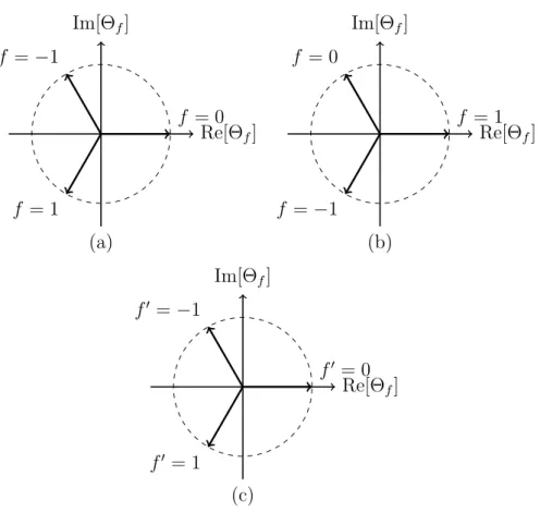
3 (f−k). (2.2) By relabeling f −k as f^′, this transformed boundary condition returns to the original one, and the boundary condition for quarks becomes invariant under the Z3 transformation. The demonstration of the FTBC in the case of k = 1 is shown in Fig. 2.1

The QCD-like theory with the boundary condition (2.1) is invariant under the Z3 transformation. This QCD-like theory is called Z3-QCD. In the zero temperature limit,Z3-QCD agrees with QCD because the temporal boundary condition is not relevant.

After the transformation

q_f →e⁻^iθ^f^{T x}⁴q_f, (2.3) the FTBC returns to the original boundary condition (1.10), and the quark part of the Lagrangian density becomes

LF,Z3 = ¯q(γ_µD_µ+ ˆM −iγ₄θTˆ )q, (2.4) where ˆθ = diag(

θ₋1, θ0, θ1

) refers the flavor-dependent imaginary chemical potential rescaled by temperature T. Obviously, because of the existence of

10

(22)

2.2. EFFECTIVE POLYAKOV-LINE MODEL 11

Re[Θ_f]

(a) Im[Θ_f]

f = 0 f =−1

f = 1

Re[Θ_f]

(b) Im[Θ_f]

f = 1 f = 0

f =−1

Re[Θ_f]

(c) Im[Θf]

f^′ = 0 f^′ =−1

f^′ = 1

Figure 2.1: Conceptual diagram of the FTBC in the case of k = 1. Here, Θ_f ≡e⁻^iθ^f. (a) The initial state. (b) The state after theZ3 transformation.

θ_f is rotated by 2π/3 in the complex plane. (c) Relabelingf−k asf^′. After that, the rotated state returns to the initial one.

θ, the flavor SU(3) symmetry is partially broken. In the massless limit ( ˆˆ M → 0), global SU(3)_V⊗SU(3)_Asymmetry is broken down to (U(1)_V)²⊗(U(1)_A)². When the chiral symmetry is spontaneously broken, the remaining symmetry is (U(1)_V)².

2.2 Eﬀective Polyakov-line model

To study the efficiency of Z3-QCD in the finite quark chemical potential region, we use the effective Polyakov-line (EPL) model [46, 50, 51]. In the temporal gauge A₄ = 0 except for a timeslice at x₄ = 0, the effective action S_P for the EPL model is determined by

e⁻^S^P =

∫

DU₄(x,0)DU_iDϕ {∏

x

δ[U_x −U₄(x,0)]

}

e⁻^S^L, (2.5)

(23)

12 CHAPTER 2. Z3 SYMMETRY AND SIGN PROBLEM where ϕ denotes the pseudofermion of boson fields, SL is the lattice action, and U_x represents the Polyakov line holonomy

U_x = diag{

eîφ^r,x, eîφ^g,x, eîφ^b,x} ,

∑3 i=r,g,b

φ_i,x = 0. (2.6) The partition function of the EPL model is written by

Z =

∫

DU exp [−S_P[U_x]], (2.7) By using Eq. (2.5), we obtain the SU(3) spin model in the three-dimensional space V =N_s³ as an eﬀective model of LQCD. In the strong coupling limit, the eﬀective gauge action becomes [50–53]

S_G=−κ∑

x

∑3 i=1

{ tr[

U_x] tr[

U^†

x+ˆi

]+ c.c.

}

, (2.8)

where κis the eﬀective coupling constant. The relation between κ and temperature T is complicated like that between the lattice coupling β and T. Thus, in order to investigate the qualitative properties of the phase struc- tures and the sign problem, we use the simple form presented in Refs. [53,54]:

the largeκcorresponds to high temperature, while the small one does to low temperature.

By using the relation Eq. (2.6), the dynamical variables for the EPL model are changed into φ_i,x. Then, the Haar measure DU becomes

DU =DφrDφg e⁻^S^H, SH =∑

x

LH(x), (2.9)

L_H(x) =−log [

sin²

(φ_r,x−φ_g,x 2

) sin²

(2φ_r,x+φ_g,x 2

)

×sin²

(φ_r,x + 2φ_g,x 2

)]

. (2.10) For the fermion action, we consider the heavy dense and the static quark.

The eﬀective action S_F is given by [55–57]

S_F =∑

x

L_F(x), L_F(x) =−2N_flog{

det [1 +h₊U_x] det[

1 +h₋U_x^†]}

=−2N_f{ log[

1 +h₊tr[U_x] +h₊²tr[U_x^†] +h³₊] + log[

1 +h₋tr[U_x^†] +h²₋tr[Ux] +h³₋]}

(2.11)

h_±=e⁽^±^µ⁻^M)/T, (2.12)

whereNf is the number of flavors, andM,µ, andT denote the heavy quark mass, the quark chemical potential, and temperature, respectively. In the

(24)

2.2. EFFECTIVE POLYAKOV-LINE MODEL 13 limit M → ∞, the Lagrangian density LF(x) is almost real when µ = M, since h₊ = 1 and h₋ → 0 in Eq. (2.11). This property is related to the particle-hole symmetry.

From the above, the partition function of the EPL model is derived by Z =

∫

DφrDφg e⁻^S^G⁻^S^F⁻^S^H, (2.13) and we call this EPLMWO, for simplicity. In this study, we consider the case of N_f = 3.

From Eq. (2.6), we can define the (traced) Polyakov line as P_x = 1

3tr[U_x] = 1 3

(eîφ^r,x+eîφ^g,x +eîφ^b,x)

. (2.14)

(In general, P_x is called the Polyakov loop, but in this study we call it the Polyakov line according to Ref. [46, 50, 51].) This quantity is not invariant under the Z3 transformation Ux → e^i2πk/3Ux (k ∈ Z), and is an order parameter of the confinement-deconfinement transition just as the case of pure SU(3) gauge theory or QCD.

2.2.1 Particle-hole symmetry

In the large mass limit, the contribution of the second term in Eq. (2.11) can be ignored, since h₋ → 0 and this term becomes constant. Therefore, we now consider only the first term in Eq. (2.11). When µ = M +δµ, the Lagrangian density becomes

L_F(x)|_µ=M_+δµ,φ_i ∼ −2N_F log[

1 +e^δµ/Ttr[U_x] +e^2δµ/Ttr[U_x^†] +e^3δµ/T]

=−6N_Fδµ/T

−2N_F log[

1 +e⁻^δµ/Ttr[U_x^†] +e⁻^2δµ/Ttr[U_x] +e⁻^3δµ/T]

=−6NFδµ/T + LF(x)|_µ=M₋_δµ,₋_φ_i. (2.15) The first term −6N_Fδµ/T doesn’t contribute the expectation values of ob- servables since it is independent of the dynamical variables φ_i. Thus, the relationL_F|µ=M+δµ,φi =L_F|µ=M−δµ,−φi is eﬀectively satisfied, and the expectation value of any quantity O without the explicit µ-dependence has the relation ⟨O(µ=M +δµ)⟩ = ⟨O(µ=M −δµ)⟩. This relation is called the particle-hole symmetry [56]. At µ=M, the Lagrangian density becomes

L_F(x)|_µ=M,φ_i ∼ −2N_F log[

1 + tr[U_x] + tr[U_x^†] + 1]

=−2N_Flog [2(1 + Re{tr[U_x]})]. (2.16) When (1 + Re{tr[U_x]})<0, the Lagrangian density (2.16) becomes complex.

However, the imaginary part is an integer multiple of 2π. Thus, the sign problem does not occur at µ=M.

(25)

14 CHAPTER 2. Z3 SYMMETRY AND SIGN PROBLEM

2.2.2 Z

³

-symmetric EPL model

In EPLMWO,Z3symmetry is explicitly broken since tr[U_x] in the Lagrangian densityL_F is not invariant under theZ3 transformation. To construct theZ3- symmetric EPL model, we introduce the flavor-dependent imaginary chemical potential iθ_fT, (θ_u, θ_d, θ_s) = (0,2π/3,−2π/3), following the manner of Z3-QCD. The corresponding Lagrangian density L_F,_Z₃(x) is derived by

L_F,_Z₃(x) = −2 ∑

f=u,d,s

log{ det[

1 +h₊e^iθ^fU_x] det[

1 +h₋e⁻^iθ^fU_x^†]}

=−2 log

{ ∏

f=u,d,s

det[

1 +h₊e^iθ^fU_x] det[

1 +h₋e⁻^iθ^fU_x^†]}

=−2 log{ det[

1 +h³₊(Ux)³] det[

1 +h³₋(U_x^†)³]}

=−2{ log[

1 +h³₊tr[(U_x)³] +h₊⁶tr[(U_x^†)³] +h⁹₊] + log[

1 +h³₋tr[(U_x^†)³] +h⁶₋tr[(U_x)³] +h⁹₋]}

. (2.17) It is easily seen that tr[(U_x)³] and tr[(U_x^†)³] are invariant under theZ3 transformation, and thus the Lagrangian density L_F,_Z₃ has the explicit Z3 symmetry. As in EPLMWO, this model also has the particle-hole symmetry.

Hereafter, we refer this model to Z3-EPLM.

For tr[(U_x)³], the (traced) cubic Polyakov line is defined by Q_x = 1

3tr[(U_x)³] = 1 3

(eî3φ^r,x +eî3φ^g,x+eî3φ^b,x)

, (2.18)

and written with P_x as

Q_x = 9{

(P_x)³−P_xP_x^∗}

+ 1. (2.19)

The cubic Polyakov line is invariant under theZ3 transformation, thus this is not an order parameter of the confinement-deconfinement transition. From the relation (2.19), it is easily seen that the degeneration between the confined stateP_x = 0 and the deconfined onesP_x = 1, e^±^i2π/3 occurs, sinceQ_x =Q^∗_x = 1 are in both states. Figure 2.2 shows the allowed regions of P_x and Q_x in the complex plane. In the left panel for P_x, both states e^±^i2π/3 are the Z3

images of the deconfined one P_x = 1.

In the complex plane of Q_x, the point Q_x = 1 corresponds to that of P_x = 0 and P_x = 1, e^±^i2π/3, as mentioned above. The origin Q_x = 0 corresponds to a configuration (φ_r,x, φ_g,x, φ_b,x) = (2π/9,−2π/9,0) and its Weyl- symmetry transformed ones. The states Q_x = e^±i2π/3, where the absolute value of Im[Q_x] is maximum and the sign problem is the severest inZ3-EPLM, correspond to configurations (φr,x, φg,x, φb,x) = (±2π/9,±2π/9,∓4π/9) and their Z3 and/or Weyl-symmetry transformed ones.

(26)

-1 -0.5 0 0.5 1

-0.5 0 0.5 1

(a)

Im[Px]

Re[P_x] P_x confnement Px deconfnementP_x severest Px

-1 -0.5 0 0.5 1

-0.5 0 0.5 1

(b)

Im[Qx]

Re[Q_x] Q_x confnement Qx deconfnementQ_x severest Qx

Figure 2.2: Allowed region of (a) P_x and (b) Q_x. The filled triangle and three vertices are the confined and deconfined states, respectively. These points degenerate at Q_x = 1 in (b). The filled circles correspond to configurations (φ_r,x, φ_g,x, φ_b,x) = (±2π/9,±2π/9,∓4π/9) and their Z3 and/or Weyl-symmetry transformed ones.

2.2.3 Fermion potential in EPL model

Here, we study properties of the fermionic Lagrangian density in EPLMWO and Z3-EPLM. For each fermionic Lagrangian density, the reality in the finite chemical potential region is not ensured, sinceP_x andQ_x are generally complex. Here, for simplicity, we discuss the sign problem in EPLMWO and Z3-EPLM with the real part of the fermionic Lagrangian density only. In the calculations, we set M/T = 10 and µ/M = 0.5,1.0 and 1.5.

Figure 2.3 shows Re[L_F] of EPLMWO in the φ_r,x–φ_g,x plane. It is seen that Re[L_F] is minimum at the configuration (φ_r,x, φ_g,x) = (0,0) corresponding to P_x = 1, and the result at µ/M = 1.5 is qualitatively the same as at µ/M = 0.5 due to the particle-hole symmetry. Thus, stochastically, the state Px = 1 is more favorable than other states. Furthermore, the Z3 images of the origin, (φ_r,x, φ_g,x) = (±2π/3,±2π/3) corresponding to P_x = e^±^i2π/3, have a lower probability thanP_x = 1, sinceZ3 symmetry is explicitly broken in EPLMWO.

Figure 2.4 shows Re[L_F,_Z₃] ofZ3-EPLM in theφ_r,x–φ_g,x plane. There are nine minimum points in both panels (a) and (c), and the result (c) is qualitatively same as the result (a). Of the nine minimum points, the configurations (φ_r,x, φ_g,x) = {(±2π/3,±2π/3), (0,0)} correspond to the deconfined states, and other six points, (φ_r,x, φ_g,x) = {(±2π/3,∓2π/3), (±2π/3,0), (0,±2π/3)}, mean the confinement configurations. From these situations, both confined and deconfined states are degenerate in this model.

Figure 2.5 shows the eﬀective potential from the Haar measureL_H in the φr,x–φg,x plane. It is clearly seen thatLH has minima at the confined states, and this result indicates that the confined states are stochastically favored

(27)

16 CHAPTER 2. Z3 SYMMETRY AND SIGN PROBLEM

(a) µ/M = 0.5

-3 -2 -1 0 1 2 3

ϕ_r,x -3

-2 -1 0 1 2 3

ϕg,x

-0.14 -0.12 -0.1 -0.08 -0.06 -0.04 -0.02 0 0.02 0.04 0.06 0.08

(b) µ/M = 1.0

-3 -2 -1 0 1 2 3

ϕ_r,x

-3 -2 -1 0 1 2 3

ϕg,x

-50 0 50 100 150 200 250 300 350 400 450

(c) µ/M = 1.5

-3 -2 -1 0 1 2 3

ϕ_r,x -3

-2 -1 0 1 2 3

ϕg,x

-90.14 -90.12 -90.1 -90.08 -90.06 -90.04 -90.02 -90 -89.98 -89.96 -89.94 -89.92

Figure 2.3: Re[L_F] in theφ_r,x–φ_g,x plane. In the calculations, we setM/T = 10 and (a) µ/M = 0.5, (b) µ/M = 1.0, and (c) µ/M = 1.5 respectively.

due to the eﬀective potential L_H.

Let us consider two models withN_s = 1, where the kinetic term is absent and the fermionic Lagrangian density L_F (or L_F,_Z₃) and L_H are dominant.

InZ3-EPLM, as mentioned above,L_F,Z₃ favors both confined and deconfined states, whileLH does the confined state. Hence, the confined state is favored inZ3-EPLM with N_s = 1.

On the other hand, in EPLMWO with N_s= 1, L_F favors the deconfined state, so that the situation is more complicated. The favored state depends on parameters. To see the dependence of parameters M and µ, we consider the following quantity

∆L_F,R = Re [L_F|Px=0−L_F|Px=1]

=−2Nf

[

log 1 +e^3(µ⁻^M)/T

1 +e^(µ⁻^M^)/T +e^2(µ⁻^M^)/T +e^3(µ⁻^M)/T + log 1 +e⁻^3(µ+M^)/T

1 +e^−(µ+M)/T +e^−2(µ+M^)/T +e^−3(µ+M^)/T ]

. (2.20) The µ/M-dependence of ∆LF,R is shown in Fig. 2.6. It is seen that ∆LF,R

becomes large around µ/M ∼ 1, while it is suppressed in µ/M < 0.5 and

(28)

(a) µ/M = 0.5

-3 -2 -1 0 1 2 3

ϕ_r,x -3

-2 -1 0 1 2 3

ϕg,x

-2x10^-6 -1.5x10^-6 -1x10^-6 -5x10^-7 0 5x10^-7 1x10^-6

(b) µ/M = 1.0

-3 -2 -1 0 1 2 3

ϕ_r,x

-3 -2 -1 0 1 2 3

ϕg,x

-20 0 20 40 60 80 100 120 140

(c) µ/M = 1.5

-3 -2 -1 0 1 2 3

ϕ_r,x -3

-2 -1 0 1 2 3

ϕg,x

-90.000002 -90.000001 -90.000000 -89.999999

Figure 2.4: Re[L_F,_Z₃] in the φ_r,x–φ_g,x plane. In the calculations, we set M/T = 10 and (a) µ/M = 0.5, (b) µ/M = 1.0, and (c) µ/M = 1.5 respectively.

µ/M > 1.5. This indicates that the deconfined state P_x = 1 is favored when ∆LF,R is large. Therefore, the deconfined state is favorably realized at µ/M ∼1.

In the EPL model with N_s > 1, the gluon kinetic term S_G exists, and this term favors the deconfined state when κ is large. Thus, at large κ, the absolute value of the spatial average of Polyakov line

P¯ ≡ 1 V

∑

x

P_x (2.21)

has a finite value. On the other hand, at small κ, the eﬀect of favoring the deconfined state is weak, and P_x is spread in the complex plane. Hence, the cancellation occurs and the spatial average ¯P becomes zero.

The relations of Re[L_F]–Im[L_F] and Re[L_F,_Z₃]–Im[L_F,_Z₃] in the case of N_f = 3 are shown in Fig. 2.7. Here, we set M/T = 10 and µ/M = 0.95, where the sign problem is considered to be serious. As for EPLMWO, in the left panel of Fig. 2.7, the maximum of |Im[L_F]| is much larger thanπ/2.