1
SummaryPrevious work in Spectral Correlation Density (SCD) estimation of cyclostationary signals has been based on the Weighted Overlapped Segment Averaging (WOSA) estimator that is known to have low resolution and high frequency leakage. In this paper we address the estimation of the SCD using the high resolution Minimum Variance Distortion-less Response (MVDR) estimator. Using the Matched Filterbank (MAFI) approach to spectral estimation we derive SCD estimators based on the classic WOSA and MVDR. The MAFI approach provides a common base that allows direct comparison between the SCD estimators and gives better insight of the relation between them. Numerical examples are presented to validate the derived estimators and to quantitatively evaluate their performance in terms of cycle frequency resolution, variance and bias of the SCD estimates.
2
IntroductionIn several engineering and science fields most signals are generated by means of periodic processes (i.e.
modulation) and as a consequence the generated signals exhibit (second order) moments that are periodic in time.
These signals are better modeled as cyclostationary and can be characterized by cyclic descriptors like the cyclic auto- correlation and spectral correlation density [2].
These cyclic descriptors are fundamental tools from where more complex cyclic descriptors can be obtained like the cyclic magnitude and cyclic phase, the cyclic coherence spectrum and the cyclic Wigner-Ville spectrum that have a rich set of practical applications in communication systems, mechanical vibration analysis, meteorology, economics, hydrology and acoustics [1, 5, 6, 7, 8, 20].
For most applications it is often more convenient and natural to analyze the structure of cyclostationary signals in the frequency domain. Therefore, it is of practical interest to estimate the spectral correlation density (SCD) from samples of the observed signal.
Most of the proposed SCD estimators in the literature are based on WOSA [9] that is well known to have poor resolution properties and large spectral leakage [1] [5].
These limitations are especially troublesome when we deal with short length observations of the signal that is a common occurrence in practical systems. The Minimum Variance Distortion-less Response (MVDR) [3, 11] has gained attention in the last decade in array processing and spectral estimation due to its higher resolution capabilities even with short length observations. In this work we argue that SCD estimation can also benefit from these high resolution properties and evaluate MVDR as a good alternative for SCD estimation.
For evaluation purposes we derive three estimators, two based on MVDR and one based on WOSA, using a Matched Filterbank (MAFI) approach [21, 16]. The MAFI approach provides a common base where each method only differs in the filters design and their bandwidth estimate.
This allows direct comparison between methods and simplifies their implementation.
In the next section we present a short review of the SCD and present a simple example of cyclostationary signal that is used later to validate the derived SCD estimators. We also formulate the SCD estimation problem as a joint spectrum estimation problem (i.e. cross spectrum) using Cyclic Demodulates. In section 4 following the MAFI
Spectral Correlation Density Estimation via Minimum Variance Distortion-less Response Filterbanks
Horacio Sanson
†and Mitsuji Matsumoto
†3-1
査読論文Refereed Papers
† Graduate School of Global Information and Telecommunication Studies
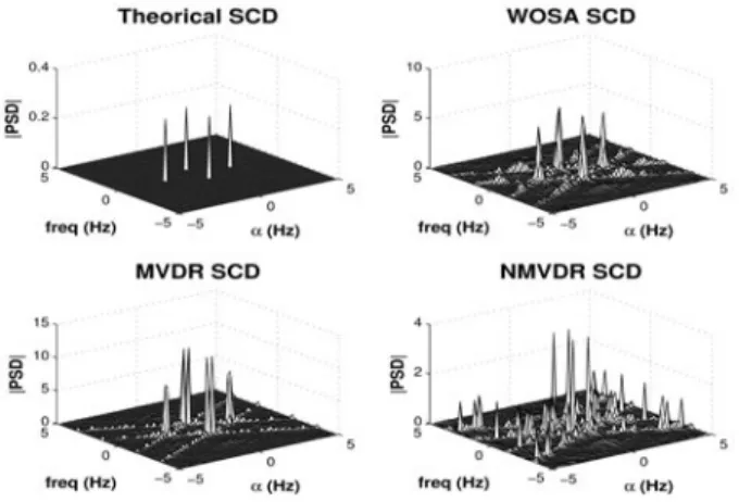
Fig. 1 Theoretical and estimated SCD.
approach, we derive cross spectrum estimators based on MVDR and WOSA and present how these estimators can be used to estimate the SCD. In section 5 we evaluate numerically the statistical properties of these estimators in terms of cycle frequency resolution, bias and variance and finally in 6 we present some discussion on the numerical results and future research work.
3
The Spectral Correlation Density A zero mean stochastic process x(n) is cyclostationary (in the wide sense) if the auto correlation function given by( , ) { ( / )} ( / )} ( )
R nx t =E x n+t 2 x n∗ −t 2 1 is periodic in time with an integer period N:
( , ) ( , ); , ( )
x x
R n t =R n lN+ t ∀n l Z∈ 2
Since the auto-correlation Rx(n,t) is periodic it accepts Fourier Series expansion and can be written as:
( , ) ( ) n ( )
x x
R n =
∑
Ra e−ia 3a
t t
where the Fourier coefficients:
( ) lim N ( , ) n ( )
x N n x
R R n e
N
−
→∞ =
=
∑
10
1 4
a t t ia
are the cyclic auto correlations and a={2pk N/ }Nk=−N are the cyclic frequencies. Note that for a=0 the cyclic correlation Rxa( )t reduces to the conventional auto correlation. As with conventional spectral analysis it can be shown that the Fourier Transform of these lag-dependent coefficients give raise to the spectral correlation density (SCD)[5]:
( ) x( ) w ( )
S w +∞ R e−
=−∞
=
∑
5a a i t
t
t
The above equation Sa(w) displays the power distribution of the signal with respect to both the spectral frequency w and the cycle frequency a. In this respect the spectral correlation density contains an additional dimension related to the non stationary features of the signal.
3.1 Spectral Correlation Properties We know from classic spectral estimation theory that the spectrum of a periodic signal with period N is also a periodic sequence with period N. Thus the support region of the spectral correlation in the plane is contained between
−p≤w=2pk/N≤p with −N/2≤k≤N/2.
Also the spectral correlation density (5) presents the following properties in the bi-frequency plane a−w [1]:
( ) ( ) ( ) ( )
S wa ∗=S w-a +a =S-a −w 6
( ) ( ) ( ) ( )
S w S w-a = a +a∗=Sa −w∗ 7
These symmetry properties in the bifrequency plane added to the periodicity in the plane restrict the frequency support of the spectral correlation to the principal quadrant of the bi-frequency plane.
3.2 Example of a Cyclostationary Signal A simple example of cyclostationary signal is an harmonic sinusoid in additive noise:
( ) ( c ) ( ) ( )
x n =Acos w n+f +v n 8
where v(n) is assumed real, stationary white noise with zero mean and variance sv2, A is a constant amplitude and wc
and f are deterministic constants in (0,p) and (−p,p) respectively. Using equation (4) and equation (5) we can derive an expression for the SCD of this model as [6, 8]:
( ) [ ( ) ( )] ( )
[ ( ) ( )] ( ) ( )
x c c
c c v
S w A w w w w
A e w e w
= − + +
+ − + + +
2
2 2 2 2
4
2 2 9
4
a
i f -i f
d d d a
d a d a s d a
For a signal with zero phase the SCD would have two peaks at (w,a)=(±wc,0) of amplitude A2/4+sv2and two peaks at (w,a)=(0,±2wc) with amplitude A2/4.
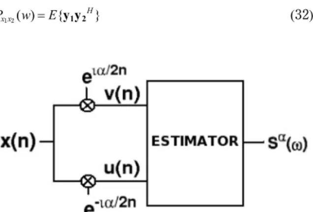
3.3 Cyclic Demodulation
To understand this interpretation we simply have to insert the auto correlation function definition given by equation (1) into (4):
( ) { ( / ) ( / )} n ( )
Rxa t =E x n+t 2 x n∗ −t 2 e−ia 10 then define u(n) and v(n) such that:
( ) ( ) n ( )
u n =x n e−i2a 11
( ) ( ) n ( )
v n =x n eia2 12
replace them in equation (10) to obtain:
( ) { ( / ) ( / )} ( )
Rxa t =E u n+t 2v n∗ +t 2 13 The equation above shows thatRxa( )t is the cross correlation of u(n) and v(n), and therefore from equation (5) follows that Sa(w) is the cross spectral density of u(n) and v(n).
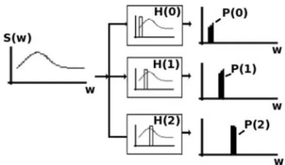
Fig. 2 Filter bank interpretation to spectral density estimation.
This interpretation suggests that Sa(w) can be estimated using any cross PSD estimator such as the WOSA and MVDR.
4
Filter bank PSD estimationThe concept of spectral estimation via filter banks is depicted in figure 2. Basically we have a zero mean signal vector xn=[ ( ), (x n x n−1), , ( x n Q− +1)]T with spectral density S(w) and pass it through a bank of narrow band filters hw=[ ( ), ( ), , (h0 h1 h Q−1)]T each one steered at a different frequency w. The output at the filters is given by:
( ) Q ( ) ( ) H ( )
q
y n −h q x n q
=
=
∑
1 − =0
n 14 h x
and the output power P(w) is:
{ }
( ) ( ) wH w ( )
P w =E y n 2 =h R hxx 15 where Rxx is an estimate of the auto correlation matrix of xn. By measuring the output power P(w) at one filter we can estimate the spectral density S(w) by the relation [12, 14]:
( ) ( ) wH w ( )
N N
S w P w
B B
= =h R hxx 16
at the frequency the filter is steered and where BN is an estimate of the effective filter bandwidth.
Based on equation (16) we can then design different S(w) estimators by choosing different filters and bandwidth parameters.
4.1 WOSA Method
The simplest filterhwcwe could design is a rectangular window of N samples with amplitude one:
[ , , , ]T ( )
= 1 11 17
h
this filter steered at a frequency w becomes:
( )
, jw, , j N w T ( )
w= 1 e e −1 18
h
and has constant bandwidth:
H ( )
N w w
B =h h =N 19
Replacing these into equation (16) we get:
( ) wH w ( )
S w =a R aNxx 20
where aw is known as the steering vector and is defined as:
( )
, jw, , j N w T ( )
w= 1e e −1 21
a
Equation (20) is the general Weighted Overlapped Spectrum Averaging (WOSA) spectral estimator. In this basic form equation (20) is equivalent to the well known periodogram:
( ) ( )
( ) ( ( )) ( )
H H
w w H
w
N jnw
n
S w N N
x n e DFT x n
N N
− −
=
= =
=
∑
=2
1 2 2
0
1 22
1 1 23
n n n
a x x a a x
By splitting the signal vector xn in segments of length Q and averaging the spectral densities of each segment we can obtain the Bartlet (Averaged Periodogram) method:
M ( )
H
M m
−
=
=
∑
10
1 24
xx m m
R x x
where M=N/Q is the number of segments and xm=[x(mQ), x(mQ−1),…,x(mQ−Q+1)]T. Using this correlation matrix the estimator becomes:
( ) ( )
( ( )) / ( )
H H
M w w
m M
m
S w M Q
DFT x m Q M
−
=
−
=
=
=
∑
∑
1
0
1 2
0
1 25
1 26
a x x am m
We could also apply windows (filter) Rxx and/or overlap the segments; operations that would result in other classic non- parametric methods of spectral estimation. During our numerical examples we won’t use any pre windows as they further degrade the already poor resolution of the WOSA method and will always use maximum overlapping of segments that presents the minimum cycle leakage for the WOSA method [1].
4.2 MVDR Method
The square filter used by WOSA has a sinc shaped impulse response H(wc) as shown in figure 3 and as we can see this shape has a direct impact in the estimate of P(wc).
To improve the estimate MVDR implements a narrow band filter with impulse response equal to unity (distortion- less) at the frequency wc while reducing as much as possible the power at the other frequency bands (minimum variance) [11].
This filter design is a well known optimization problem where we solve forhwc by minimizing the power:
H ( )
wc= wc xx wc 27
h h R h
Fig. 3 Spectral density estimation via filtering.
subject to the constraint hwcHa=1where a is the steering vector defined in (21).
This optimization problem has a known solution given by [3, 11]:
( )
w
−
= − 28
c xx1
H 1
xx
h R a a R a
replacing this in (15) gives the PSC (Power Spectrum Capon) estimator:
( )c ( )
P w = H1−1 29
a R axx
To get S(wc) we must normalize P(wc) by the filter bandwidth BN as per relation (16). A simple estimate of BN is given by the reciprocal of the filter length, that is BN=1/Q, that results in the MVDR estimator [3]:
( ) ( )
MVDR c Q
S w = H −1 30
a R axx
Another estimator known as normalized MVDR or NMVDR is obtained by using the relation BN=aHa that results in [13]:
( ) ( )
NMVDR c
S w = HH −−xx12 31
xx
a R a a R a
We can see from equations (30) and (31) that both MVDR and NMVDR are adaptive filters as they depend on the signal features Rxx. This is in contrasts with the rectangular filter used by WOSA that is generic and does not consider the signal to be filtered in its construction.
4.3 Cross Power Spectrum Estimation and SCD Estimation.
From a filtering point of view the estimation of the cross power spectrum from two data vectors x1 and x2 can be based on the design of two narrow band pass filters hx1
and hx2steered at the same frequency wc. Therefore the cross power spectrum can be inferred as the cross correlation of the filter outputs at lag zero [14]:
( ) { H} ( )
Px x1 2 w =E y y1 2 32
where y1 and y2 are the filter outputs given by hx1Hx1 and
H x2 2
h x respectively. Using (16), (20), (30), (31) and (32) we can easily find:
( ) ( )
( ) ( )
( ) ( )
wH w
WOSA
wH w
MVDR H H
w w w w
wH w
NMVDR H
w w
S w
Q
S w Q
S w
− −
− −
− −
− −
=
=
=
33
34
35
1 2
1 1 1 2 2 2
1 1 2 2
1 1 1 2 2 2
1 1 2 2
x x
1 1
x x x x x x
1 1
x x x x
1 1
x x x x x x
1 1
x x x x
a R a
a R R R a a R a a R a a R R R a
a R R a
where, Rx1x1, Rx2x2, and Rx1x2 are the Q x M auto correlations and the cross correlation respectively of the signal vectors.
Using these cross spectrum estimators we are now able to obtain an estimate of Sa(w) using the cyclic demodulation procedure described in section 3.3 and shown in figure 4.
The procedure is as follows: for each cyclic frequency a of interest we shift x(n) by a step size ±a/2 to obtain expressions (11) and (12) and use these frequency shifted versions of x(n) as inputs to any of the cross PSD estimators (33), (34) or (35). The output of this is the estimated Sa(w) at the respective cyclic frequency a.
5
Numerical EvaluationIn the discussion that follows we present the bias, variance and cyclic resolution properties of the SCD estimators presented in section 4.3 with different segment sizes for WOSA and different filter lengths for MVDR and NMVDR. We will refer to each test case with the method name followed by the segment or filter lengths (i.e. WOSA Q).
For WOSA the values of Q represent segment size and take the values N, N/2 and N/4 where N is the total number of samples of the signal. As mentioned above WOSA N is the known periodogram used extensively in classic spectral estimation. For MVDR and NMVDR Q represents the filter lengths and has a maximum value of N/2 because larger values would cause Rxx to be singular (i.e. non invertible) that would result in unstable spectral estimates.
In all simulations we generated 64 samples of the example signal presented in section 3.2 with a signal frequency of fc=1.5Hz and sampled at 10Hz.
To simplify our numerical results we set the amplitude to A=1. Also based on the periodic and symmetric properties of the spectral correlation (section 3.1) we only estimate the first quadrant of Sa(w) in the bi-frequency plane a−w and obtain the other three quadrants using the symmetry properties. This greatly reduces the computation time and memory consumption of our algorithm.
Before we can estimate Sa(w) using any of our derived estimators (33), (34) or (35) we need to estimate Rxx first.
We have the forward estimate:
Fig. 4 SCD Estimation via cyclic demodulates Method.
ˆF N ( ) ( ) ( )
n
R x n x n
N
− ∗
=
=
∑
10
1 36
or the forward-backward sample estimate:
ˆˆˆFB (ˆF ˆFT ) ( )
R 1 R JR J 37
2
where J is the reflection matrix. We prefer to use the forward-backward sample estimate as it is known to have better statistical properties than the forward-only estimate [10, 17].
5.1 Probability of cyclic resolution
We are interested in evaluating the probability of resolution of the cyclic frequency that is characteristic of the SCD.
Although there is no rigorous definition of cyclic frequency resolution we can define a resolution criterion as the frequency separation ∂a=a1−a2 at which the SCD evaluated at am=(a1+a2) /2 is equal to the average of the
SCDs evaluated at a1 and a2 [19, 22]:
( ) { ( ) ( )} ( )
S m w =1 S w S w1 + 2 38
2
a a a
Using this criterion we can establish a random inequality to define a resolution event:
( , ) (S w S w( ) ( )) S m( )w ( )
Γ 1 2 =1 1 + 2 − >0 39
2 a a a
a a
Correspondingly we can define the binary probability of resolution Pres as [22]:
( ) ( )
Pres=P Γ >0 40
To evaluate the probability of resolution we generated two signals using the same parameters but with frequencies wc
and wc+ ∂a where ∂a takes values from 0Hz to 1Hz in steps of 0.05Hz. This two signals added together result in a SCD similar to those in figure 1 with four additional peaks at:
( , ) (w a = ± + ∂wc a, )0
Fig. 5 Probability of resolution.
Fig. 6 Bias of the WOSA SCD estimator.
���� ��� ��� �� � � �� �� ��
�
�
�
��
��
��
��
��
��
��
��������������������������
����
������������������������������
������
��������
��������
Fig. 7 Bias of the WOSA MVDR estimator.
���� ��� ��� �� � � �� �� ��
�
�
�
�
�
�
�
�
��
��������������������������
����
������������������������������
��������
��������
��������
Fig. 8 Bias of the WOSA NMVDR estimator.
��� ��� ��� �� � � �� �� ��
���
���
���
��
�
�
��
��
��
��������������������������
����
�������������������������������
���������
���������
���������
and
( , ) ( ,w a = 0 2± (wc+ ∂a)).
In figure 5 we plotted the probability of cyclic resolution P(Γ >0) of the two peaks at (0,wc) and (0,2(wc+ ∂a)) as a
function of the cyclic frequency separation ∂a.
As seen in the figure, all test cases present a threshold effect where the probability of resolution is zero until the smaller ∂a resolvable by each test configuration is reached.
At this threshold point all methods, except for NMVDR N/8, rapidly achieve 100% probability of resolution of the two peaks.
All methods of the same segment/filter size have similar probability of resolution marked by the circular regions in the plot. In all three circular lines NMVDR presents the best resolution followed by MVDR and finally WOSA. As segment/filter length increases all three methods improve in resolution capability but even with no averaging (WOSA N) WOSA lacks behind NMVDR N/4 in resolution.
This high resolution property, when compared to WOSA, is one of the praised strengths of the MVDR and NMVDR estimators and as we can see cyclic spectral analysis also benefits from this high resolution property.
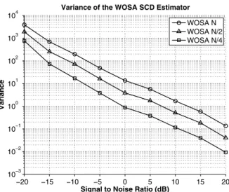
5.2 Bias and Variance
To obtain the bias and variance of the SCD estimators we estimated the SCD at the point (w,a)=(0,2wc) over a range of SNR values from −20dB to +20dB using different segment sizes for WOSA and filter lengths for MVDR and NMVDR estimators. For each value of SNR we repeated the experiment over 200 independent trials while accumulating the bias, variance and minimum squared error (MSE) of the spectrum magnitude estimates.
From the bias plots 6, 7 and 8 we can see that all estimators are biased with WOSA N having the largest bias.
For segments sizes and filter lengths below N/4 we find that MVDR and WOSA estimators presents similar bias while NMVDR goes to both extremes, it has the lowest bias at N/8 but quickly increases for larger filter lengths
In the variance plots 9, 10 and 11 we see that WOSA and MVDR, as with the bias, present a similar behavior that improves as the SNR increases and with MVDR slightly better than WOSA. Also as with the bias, NMVDR has the lowest variance at N/8 but also presents a quick degradation for larger filter lengths and SNR values.
To make an overall performance comparison between the estimators we plotted their Minimum Square Error (MSE) in Fig. 11. WOSA N/2, MVDR N/2 and WOSA N/4, MVDR N/4 present very similar performance as seen also in the bias and variance plots. These performance similarities appear because MVDR can be though as an adaptive version of the WOSA method. To see this it suffices to replace −1 1
x x1
R and −2 2 x x1
R in (34) with the identity matrix I and it will reduce to the WOSA estimator (33) [15].
NMVDR has the lowest MSE with short filter length but the performance degrades significantly as larger filters are used. Again we can see a trade-off in performance vs.
Fig. 9 Variance of the WOSA SCD estimator.
��� ��� ��� �� � � �� �� ��
����
����
����
���
���
���
���
���
��������������������������
��������
����������������������������������
������
��������
��������
Fig. 10 Variance of the MVDR SCD estimator.
��� ��� ��� �� � � �� �� ��
����
����
����
���
���
���
���
���
��������������������������
��������
����������������������������������
��������
��������
��������
Fig. 11 Variance of the NMVDR SCD estimator.
��� ��� ��� �� � � �� �� ��
����
����
���
���
���
���
��������������������������
��������
�����������������������������������
���������
���������
���������
segment/filter lengths as seen in the probability of resolution but in the opposite direction. Increasing lengths improves resolution but degrades the MSE performance while decreasing lengths improves MSE but reduces resolution.
6
Conclusions and Future WorkFor applications that require to separate very closely spaced frequency components and do not care about the accuracy of the estimated spectrum magnitude the NMVDR would be the best candidate as it presents the best resolution. In most situations where less resolution is tolerable the MVDR method is a better candidate over the classic WOSA method as it has better resolution and comparable bias and variance. In more stringent applications it is possible to use the high resolution of NMVDR to locate the cyclic frequency bin positions and then use MVDR or the less complex WOSA to obtain SCD magnitude at those bin positions only. This way we may get the best SCD estimate by combining the properties of these estimators at the cost of higher computational cost.
As noted by others [4, 18] the high bias and variance presented by the NMVDR is caused by an over estimated bandwidth BN. We could improve the SCD estimates by selecting a better BN but care must be taken that such bandwidth values may result in an increased complexity with a little or no improvement on the final spectral density estimate [12].
Our numerical results show that both MVDR and NMVDR exceed in resolution the classic WOSA method and in the case of the MVDR a small improvement in variance and bias. This suggests that MVDR is a better candidate for SCD estimation. Further research will concentrate in efficient implementations of the MVDR and NMVDR methods to reduce the high computational cost mostly due to the matrix inversion.
Finally we must say that these empirical experiments
where designed to test the capacity of the estimators to estimate the SCD of a simple cyclostationary signal and for that they are not exhaustive and analytical studies are required to obtain more compete results.
7
Bibliography[1] J. Antoni. Cyclic spectral analysis in practice.
Mechanical Systems and Signal Processing, 21:
597-630, February 2007.
[2] R. Boyles and W. Gardner. Cycloergodic properties of discrete- parameter nonstationary stochastic processes. IEEE Transactions on Information Theory, 29(1): 105, 114, January 1983.
[3] J. Capon. High-resolution frequency wavenumber spectrum analysis. Proceedings of the IEEE, 57(8):
1408-1418, April 1969.
[4] Wang Chengyi and Wang Hongyu. Estimation of cyclic spectra using maximum likelihood filters.
Fourth International Conference on Signal Processing Proceedings, 1: 39-42, 1998.
[5] W. Gardner. Measurement of spectral correlation.
IEEE Transactions on Acoustics, Speech, and Signal Processing, 34(5): 1111-1123, October 1986. [6] W. Gardner. Spectral correlation of modulated
signals: Part i-analog modulation. IEEE Transactions on Communications, 35(6): 584-594, June 1987. [7] W. Gardner, W. Brown, and Chen Chih-Kang.
Spectral correlation of modulated signals: Part ii-digital modulation. IEEE Transactions on Communications, 35(6): 595-601, June 1987. [8] Georgios B. Giannakis. Digital Signal Processing
Handbook, chapter 17. CRC Press, February 1999.
Digital Signal Processing Handbook.
[9] G. Heinzel, A. Rudiger, and R. Schilling. Spectrum and spectral density estimation by the discrete fourier transform (dft), including a comprehensive list of window functions and some new flat-top windows.
Technical report, Albert Einstein Institut, Teilinstitut Hannover, February 2002.
[10] M. Jansson and P. Stoica. Analysis of forward-only and forward-backward sample covariances. IEEE Transactions on Acoustics, Speech, and Signal Processing, 1999.
[11] R. T. Lacoss. Data Adaptive Spectral Analysis Methods. Geophysics, 36: 661-675, 1971.
[12] M. Lagunas and A. Gasull. An improved maximum likelihood method for power spectral density estimation. IEEE Transactions on Acoustics, Speech, and Signal Processing, 32(1): 170-173, February 1984.
[13] M. Lagunas and A. Gasull. Measuring true spectral density from ml filters (nmlm and q-nmlm spectral Fig. 12 MSE of SCD Estimators.
−20 −15 −10 −5 0 5 10 15 20
10−1 100 101 102 103 104 105
Signal to Noise Ratio (dB)
MSE
MSE Comparison of SCD Estimators
WOSA N WOSA N/2 WOSA N/4 MVDR N/2 MVDR N/4 MVDR N/8 NMVDR N/2 NMVDR N/4 NMVDR N/8
estimates. IEEE International Conference on Acoustics, Speech, and Signal Processing, 9: 608- 611, March 1984.
[14] M. Lagunas, M. Santamaria, A. Gasull, and A.
Moreno. Cross spectrum ml estimate. IEEE International Conference on ICASSP, 10: 77-80, April 1985.
[15] E. G. Larsson, J. Li, and P. Stoica. High-resolution nonparametric spectral analysis: theory and applications, chapter 4. High-Resolution Signal Processing. NY: Marcel-Dekker, New York, 2003. [16] E. G. Larsson, P. Stoica, and J. Li. Spectral estimation
via adaptive filterbank methods: a unified analysis and a new algorithm. Signal Process., 82(12): 1991- 2001, 2002.
[17] H. Li, J. Li, and P. Stoica. Performance analysis of forward-backward matched-filterbank spectral estimators. IEEE Transactions on Signal Processing, July 1998.
[18] H. Li, P. Stoica, and J. Li. Capon estimation of covariance sequences, 1998.
[19] L. Marple. Resolution of conventional fourier, autoregressive, and special arma methods of spectrum analysis. ICASSP ’ ., 2: 74-77, May 1977.
[20] Erchin Serpedin, Flaviu Panduru, Ilkay Sari, and Georgios B. Giannakis. Bibliography on cyclostationarity. Signal Process., 85(12): 2233- 2303, 2005.
[21] P. Stoica, A. Jakobsson, and J. Li. Matched-filter bank interpretation of some spectral estimators.
Signal Processing, April 1998.
[22] Q. T. Zhang. Probability of resolution of the music algorithm. Signal Processing, IEEE Transactions on Acoustics, Speech, and Signal Processing, year =, 43(4): 978-987, April 1995.