芝浦工業大学学術リポジトリ

(1)

Improvement of Energy and Control

Performance in Water Hydraulic Transmissions

by PHAM, Ngoc Pha

Dissertation submitted to the Functional Control Systems,

Graduate School of Engineering at

Shibaura Institute of Technology

in partial fulﬁlment of the requirements for the degree of

Doctor of Engineering

(2)

(3)

Acknowledgements

This research has been performed at the Environmental Systems Control Laboratory, Department of Machinery and Control Systems, College of Systems Engineering and Science, Shibaura Institute of Technology, Japan, under the supervision of Prof. Kazuhisa Ito. First and foremost, I would like to express my deeply gratitude to Prof. Kazuhisa Ito for his whole-hearted guidance and support. I also extend my sincere thanks to Prof. Shigeru Ikeo, Department of Engineering and Applied Sciences, Sophia University for proving kind help and support when I did experiment at his university.

My deepest gratitude is due to the staﬀs of all associated departments who made my study possible from the initial to ﬁnal stages.

I am grateful to all my dear Japanese friends from Environmental Systems Control Laboratory, Shibaura Institute of Technology, for their unlimited supports.

Especially, I would like to give my special thanks to my family who gave me tremendous spiritual encouragements.

(4)

Abstract

(5)

List of Figures

1.1 Hydraulics application trends and key milestones [1]. . . . 4

1.2 Trend in turnover of Danfoss Nessie Group for water hydraulics [1]. 5 1.3 Water hydraulic waste packer lorry [1]. . . . 7

1.4 Self-propelled water hydraulic vehicle [2]. . . . 7

1.5 1750 ton roof support with 480 mm bore leg cylinder – note the bronze plated rods [3]. . . . 8

1.6 Roof support for 7 m face with 500 mm bore leg cylinders [3]. . . . 8

1.7 Tap water hydraulic driven burger-machine [1]. . . . 9

1.8 Ice fill machines for 400 ices per minutes [1]. . . . 10

1.9 Automatic control tobacco cutter machine driven by water hydraulics with two cylinders [1]. . . . 11

1.10 Water hydraulics drives for wing press equipment for an aero plane factory [1]. . . . 12

1.11 Water versus bio oil, mineral oil and emulsions [1]. . . . 13

1.12 Power losses of servo systems: (a) Conventional system, (b) Variable pressure system, (c) Variable flow system, and (d) Load sensing system [4]. . . . 16

2.1 Schematic of water hydraulic FST System. . . . 21

2.2 Supply response. . . . 22

2.3 Control valve circuit for all systems. . . . 22

2.4 Control valve circuit with load. . . . 23

2.5 Model of axial piston pump. . . . 24

2.6 Model of relief valve [5]. . . . 27

(9)

LIST OF FIGURES

2.8 Modeling of P/Q characteristic of relief valve. . . . 28

2.9 Component of a bladder type accumulator. . . . 29

2.10 Operation of ON/OFF Valve. . . . 31

2.11 Component of ON/OFF Valve. . . . 32

2.12 Turbulent flow through an orifice. . . . 33

2.13 Modeling of opening area of ON/OFF Valve. . . . 34

2.14 Control logic of ON/OFF valves. . . . 37

2.15 Experimental results of flywheel velocity (ωref = 800 min−1). . . . 41

2.16 Experimental result of flow rate q2 (ωref = 800 min−1). . . . 42

2.17 Experimental and simulated results of flywheel velocity (ωref = 800 min−1). . . . 43

2.18 Pressure p2 response in experiment. . . . 45

2.19 Experimental results of percentage error emin. . . . 46

2.20 Experimental results of percentage error emax. . . . 47

2.21 Experimental results of percentage error emin. . . . 48

2.22 Experimental results of percentage error emax. . . . 48

2.23 Velocity responses in Cases 1 and 2 (ωr = 800 min−1). . . . 49

2.24 Velocity responses in Cases 2, 3 and 4 (ωr= 800 min−1). . . . 50

2.25 Pressures: (a) p2.i (i = 1, 2) and (b) p3.i (i = 1, 2) in Cases 1 and 2 (ωr = 800 min−1). . . . 50

2.26 Percentage errors: (a) emin and (b) emax in four cases. . . . 54

2.27 Pressure p1.i in four cases (ωr = 800 min−1). . . . 54

2.28 Energy consumptions in four cases. . . . 56

2.29 Supply power to the electric motor M in four cases (ωr = 800 min−1). 57 2.30 Supply pressure ps.i in four cases (ωr = 800 min−1). . . . 57

2.31 Flow rate Q2.1 in Case 1 (ωr = 800 min−1). . . . 59

2.32 Recovered energies in four cases. . . . 60

2.33 Estimation of saved energy in Case 1 (ωr = 800 min−1): (a) velocity responses in cases of using only electric or saved energy, (b) estimation of saved energy. . . . 61

(10)

LIST OF FIGURES

2.35 Estimation of saved energy in Case 3 (ωr = 800 min−1): (a)

velocity responses in cases of using only electric or saved energy,

(b) estimation of saved energy. . . . 63

2.36 Estimation of saved energy in Case 4 (ωr = 800 min−1): (a) velocity responses in cases of using only electric or saved energy, (b) estimation of saved energy. . . . 64

2.37 Net energy consumptions in four cases. . . . 65

3.1 Schematic of water hydraulic PMT system. . . . 70

3.2 Frequency converter input-output mapping. . . . 71

3.3 Control structure of PMT system. . . . 72

3.4 Velocity response of the PMT system (ωwr = 800 min−1). . . . 73

3.5 Control signal of electric motor. . . . 74

3.6 Supply power to the electric motor M. Blue line – ωr= 600 min−1, green line – ωr = 700 min−1, red line – ωr = 800 min−1, cyan line – ωr = 900 min−1, violet line – ωr= 1000 min−1 . . . 75

3.7 Estimation of saved energy of the PMT system (ωr = 800 min−1): (a) velocity responses in cases of using only electric or saved energy, (b) estimation of saved energy. . . . 76

3.8 Net energy consumption of FST, PMT and relative wasted energy of FST. . . . 79

4.1 Schematic of the water hydraulic SMS. . . . 83

4.2 Velocity response of FST, PMT, and SMS (ωr = 800 min−1). . . . 84

4.3 Percentage errors: (a) emin.i, (b) emax.i of FST, PMT, and SMS . 86 4.4 Electric power supplied to the electric motor M of FST, PMT, and SMS (ωr= 800 min−1). . . . 89

4.5 Supply pressure ps.i of FST, PMT, and SMS (ωr = 800 min−1). . 89

4.6 Working pressure p1.F and p1.P for FST and PMT (ωr = 800 min−1). 89 4.7 Net energy consumption of FST and PMT systems and energy consumption of SMS. . . . 92

B.1 Diagram of a high pressure water cleaner [1]. . . . 101

(11)

LIST OF FIGURES

B.3 Humidification control in green house [1]. . . . 102 B.4 Wood processing for sawmills [1]. . . . 103 B.5 control Process for lumber drying in a kiln [1]. . . . 103 B.6 Fire fighting by high pressure water hydraulics for generation of

(12)

List of Tables

1.1 Disadvantages of water hydraulics [2]. . . . 14

1.2 Overall average efficiency of valve-controlled hydraulic crane [4]. . 17

2.1 Valve operation logic in Phase 2. . . . 37

2.4 Control performance of rotational velocity. . . . 41

2.5 Control performance of rotational velocity. . . . 43

2.6 Velocity error of various reference velocities with conversion time of 300 ms. . . . 46

2.7 Velocity error of various reference velocities with conversion time of 300 ms. . . . 46

2.8 _{Number of valve switching in two cases (ωref = 800 min}−1). . . . 49

2.9 Velocity responses in four cases. . . . 52

2.10 Energy consumptions in four cases. . . . 56

2.11 Recovered energies in four cases. . . . 59

2.12 Saved energy in four cases. . . . 63

2.13 Net energy consumptions in four cases. . . . 66

3.1 Experimental velocity response of the PMT system. . . . 73

3.2 Energy consumption of the PMT system. . . . 74

3.3 Saved energy of the PMT system. . . . 77

3.4 Net energy consumption of the PMT system. . . . 78

(13)

LIST OF TABLES

3.6 Wasted energy indexes. . . . 80

4.1 Transient responses of FST, PMT, and SMS. . . . 85

4.2 Steady-state responses of FST, PMT, and SMS. . . . 85

4.3 Energy consumption of FST, PMT and SMS. . . . 90

4.4 Net energy consumption of FST and PMT systems and energy consumption of SMS. . . . 91

A.1 Specifications of experimental devices . . . . 98

(14)

Nomenclature

Roman Symbols

A The area of the piston bore

A0 The cross section area of an oriﬁce

Ah The heat transfer area of the accumulator

Amax The maximum opening area of an ON/OFF valve AON/OFF The cross section area of an ON/OFF valve

Cv The speciﬁc heat at constant volume of the internal gas

D The diameter of the cycle of bore center of the hydraulic pump d The diameter of the bore the hydraulic pump

d0 The diameter of an oriﬁce

Econ.PMT The total energy consumption of the PMT Econ.i The total energy consumption in Case i

emax The percentage for error of maximum rotational velocity emin The percentage for error of minimum rotational velocity Enet.PMT The net energy consumption of PMT

(15)

NOMENCLATURE

Ere.i The recovered energy to the accumulator ACC2 in Case i Esave.PMT The saved energy of the PMT

Esave.i The saved energy in Case i

Ewaste The relative wasted energy of FST to PMT

f The frequency of electrical power supply to the electric motor Gm The reference model

GP c The transfer function of PID controller for PMT

GSc The transfer function of PID controller for servo motor system

h The heat transfer coeﬃcient into the accumulator h The stroke length of the piston of the hydraulic pump IPM The moment of inertia of the hydraulic pump/motor KP D The derivative gain of the PID controller for PMT

KP I The integral gain of the PID controller for PMT

KP P The proportional gain of the PID controller for PMT

KSD The derivative gain of the PID controller for servo motor system

KSI The integral gain of the PID controller for servo motor system

KSP The proportional gain of the PID controller for servo motor system

m The mass of the gas inside the accumulator

n The rotational velocity of the driven shaft of the hydraulic pump P The number of poles of the electric motor

(16)

NOMENCLATURE

pACC2.i The pressure of the ﬂuid inside the accumulator ACC2 PM The number of poles of the electric motor

P OF The percentage overshoot of the FST system

P OP The percentage overshoot of the PMT system

P OS The percentage overshoot of servo motor system

QP The ﬂow rate of the hydraulic pump

Qh The heat energy transferred into the accumulator

QACC2.i The ﬂow rate charged into the accumulator ACC2 in the deceleration processes corresponding to Case i

QON/OFF The flow rate through an ON/OFF valve Qorifice The flow rate through an orifice

R The ideal gas constant

T The time constant of an ON/OFF valve

Tg The temperature of the gas inside the accumulator

Tw The temperature of the accumulator wall

tw The operation time in Phase 1 and Phase 2

tend The time at the end of a cycle TPM,L The load torque of the motor

tstart The time at the beginning of a cycle u The internal energy per unit of mass

(17)

NOMENCLATURE

W The external work of the accumulator z The number of cylinders

Greek Symbols

α The title angle

αd The discharge coeﬃcient of an oriﬁce

∆PHL The pressure diﬀerence between the high/low pressure ports of the

hydraulic pump/motor

∆PON/OFF The pressure diﬀerence of input/output ports of an ON/OFF valve

∆POrifice The pressure diﬀerence between input/output ports of an oriﬁce ηPMT The saved energy index of the PMT

ηPM The volumetric eﬃciency of the motor

ηP The volumetric eﬃciency of the hydraulic pump

ηw The ratio between the relative wasted energy and net energy consumption

of FST

ωmax The maximum velocity in the constant Phase ωmin The minimum velocity in the constant Phase ωref The reference velocity

ρ The ﬂuid density

τ The thermal time constant of the accumulator

τa The thermal time constant when all the gas was released

τn The time constant of the electric motor

ε The frequency coeﬃcient

(18)

Chapter 1 Introduction

1.1 Water Hydraulics

1.1.1 Historical View

Water hydraulics has a long history [6]; however, water hydraulic system did not have an important position in industry until recent years when the world faces environmental pollution, industrial wastes, unsafe situation in some specification fields such as coal extraction, food processing, etc. Because of these benefits, water hydraulics is considered as the future drive system. The brief development of water hydraulic systems will be introduced in the following section.

Water hydraulics has a very early starting point, almost all investigators agreed that the ideas and the tangible “hydraulic”devices produced by the Greeks of 5th century BC onwards. However, until Aristotle (384 BC – 322 BC) who regarded as the ﬁrst person laid the foundation for researching academically on water with his postulate “water is a continuum”, water hydraulic started studying naturally. Aristotle was also respected with the title “Father of Hydraulics”.

The application of water considered as the ﬁrst mechanical system was made by Egyptian named Ktesibios in about 250BC. It is a very simple musical instrument - water powered organ that remained the standard for such instrument until late Middle Ages.

(19)

1.1 Water Hydraulics

mathematically that the pressure at a point in a fluid at rest is equal from all sides. For his work in the field of fluid power the S.I. unit of pressure bears his Pascal’s name. The first industrial application of the hydraulic press (using water as the working fluid) based on Pascal’s theory was performed later on by Josef Bramah (1748 – 1814), in 1795, in London.

Following the invention of the steam engine by James Watt (1736 – 1819), hydrostatic machines were widely used in England for energy exchange in the form of pressurized water network. Pumps driven by steam engines were employed to generated pressurized water, which was in turn used to actuate pistons driving the processing machines.

In the second half of the 19th century, William George Armstrong (1810 – 1900) developed many hydrostatic machines and devices, primarily for use in shipbuilding. Some of these control devices still resemble those used today.

Fluid power technology has then developed mainly from the beginning of the 20th _{century. Early 20}th _{century, Professor Harvey D William, professor of}

Engineering at Cornell University began work on a new design of pump/motor combination. He and an American engineer named Reynolds Jenney cooperated to develop the first variable hydrostatic transmission, something the hydraulic industry really needed. Williams and Jenney’s development was the first hydraulic components requiring the medium to be an efficient lubricant. This was the one requirement to make oil had important position in hydraulic field. Another requirement to make oil hydraulic gained its major role is avoiding leakage because of poor quality of seals.

In 1940’s, it marked the huge increase in use of oil hydraulic because of demand of heavy presses, particularly of forging presses, demand of aircraft and marine application. However, after an accident concerning with use of oil hydraulic system in a coal mine in Belgium called Bitter Heart Mine in the summer of 1956, the use of oil hydraulic system in some speciﬁc and dangerous areas was limited, and water hydraulic presented many outstanding advantages in such areas.

(20)

technologies are required urgently. From late 1990’s, water hydraulic drive systems were developed and considered as the 4th driving source.

1.1.2 Modern Water Hydraulics

1.1.2.1 The Development of Water Hydraulics

Nowadays, the most important requirement for technical application is that the systems and devices need to be safe, clean, and environmental friendly; from this point of view, water hydraulics that uses pure tap water as pressure medium emerges as an important solution and it is considered as the fourth driving source beside electricity, pneumatics, and conventional oil hydraulics, especially in the ﬁeld of food and medicine processing, steel and glass production, ocean exploration, under water robotics [7], nuclear power generation [8], under water gait-training orthosis [9], wave and wind power generation systems, and mining machinery [10].

Water hydraulic has a very long story as mentioned in [6]; however, it has been paid much attention by researchers only since late 1990s because of the limitations including oxidation and rust, poor lubricity, low viscosity of water, bacterial growth, and particles contaminants present as shown and indicated the remedies in [1,2]. Recencly, advances in material and machining technology bring longer lifetime, higher ﬂow rate and pressure for water hydraulic components [11] and especially, current researches on the improvement of water hydraulic devices such as pumps [7,12,13], valves [10,14,15], and actuators [16,17,18] or other studies on tribology of materials under water lubrication [19] even in high temperature and pressure [20] bring a bright future and wider applications for water hydraulics.

(21)

The turning point came in 1994, when Danfoss introduced the ﬁrst generation of modern tap water components known as the Nessie⃝ family of products forR

high-pressure tap water hydraulic systems that operate typically up to 140 bar. Since 1997 Danfoss has introduced such a second generation of low-pressure and low-power tap water hydraulic components that operate up to 50 bar.

Figure 1.1: Hydraulics application trends and key milestones [1].

(22)

Figure 1.2: Trend in turnover of Danfoss Nessie Group for water hydraulics [1].

Institutions interested in modern water-hydraulics are listed as: Institute of Hydraulics and Automation, Tampere University of Technology, Finland, Linkoping University, Sweden, Department of Control and Engineering Design, Technical University of Denmark, University of Wales, Cardiﬀ, Fluid Power Center, University of Bath, Tohoku University, Sophia University, Shibaura Institute of Technology, the State Key Laboratory of Fluid Power Transmission and Control, Zhejiang University, China, Huazhong University of Science and Technology, China, and School of Mechanical and Production Engineering, Nanyang Technological University, Singapore.

(23)

1.1.2.2 Application of Water Hydraulics

This subsection introduces various applications of water hydraulics, the applications were mentioned in some published conference paper such as [1,2,3].

Water hydraulic mobile machines

All hydraulic functions for lifting and ﬁlling on the designed Waste Packer Lorries for Gothenburg Municipal, Sweden are shown one of them in Fig. 1.3. The functions are controlled and operated by water hydraulics to protect the environment in the city. The beneﬁts are no risk of oil spill drops or product contamination, and easy to clean. The vehicles have el-hybrid motors.

Figure1.4 shows a self-propelled water hydraulic vehicle developed at Purdue University. In this project the original oil hydraulic system was replaced with one using water hydraulic components. This vehicle was primarily developed in order to provide an alternative diﬀerent than oil for the equipment used for maintaining the expensive and delicate grass of golf courses.

Water-based hydraulic systems for longwall mining roof supports

Water hydraulics is very useful for protecting from ﬁre hazard. Thus, it has been used successfully for many years in self-advancing hydraulic roof supports for the longwall mining of minerals such as coal and potash. Some examples of the largest and latest roof supports, or shields are shown in Figs. 1.5 and 1.6. The coal face consists of a line of around 150 of these supports, which support the roof of the mine whilst the shearer cuts the coal along a face length of around 300 m. The operation of such a modern longwall face is now highly automated.

Tap water hydraulic machinery designed for hygiene

(24)

Figure 1.3: Water hydraulic waste packer lorry [1].

(25)

Figure 1.5: 1750 ton roof support with 480 mm bore leg cylinder – note the bronze plated rods [3].

(26)

lighter weight of cutting tools (saws etc.) due to higher power density, much higher eﬃciency and saving energy costs. A tap water hydraulic driven meat burger-machine is shown in Fig.1.7. A motor is driving the spindle for the meat cutting of beef meat, and two water cylinders for motion control are used to form the ﬁve meat burgers in one row, and one cylinder for moving the forming tool horizontally. The machine is very environmentally friendly and very easy to clean daily.

Figure 1.7: Tap water hydraulic driven burger-machine [1].

An automatic controlled ice ﬁll machine for Tetra Pak Hoyer in Denmark with a capacity of 400 ices per minutes driven by electro water hydraulics with one motor, 3 linear servo cylinders and 3 end cylinders is shown in Fig. 1.8.

An automatic control tobacco cutter machine for Universelle Germany is shown in Fig.1.9with two water hydraulic cylinders to avoid no risk of pollution, easy cleaning and save energy.

(27)

(28)

(29)

(30)

1.1.3 Advantages and Disadvantages of Water Hydraulics

According to [1, 2, 21], the benefits of water relative to mineral oil, bio oil and water-oil emulsion are illustrated in Fig. 1.11. The significant advantages and benefits can be listed as follows:

• No pollution of the environment (since most processes create leakage and ﬂuid spills).

• Low operational and power media costs, i.e. purchase, storage, disposal • Non-ﬂammable explosion-proof ﬂuid, safe and suitable for use in hazardous

applications (lower insurance costs, require less cooling capacity etc.) • High ﬂuid power density, high power eﬃciency and high torque to inertia

ratio compared to electric drives and pneumatic drives.

• Workers do not breathe harmful oil vapors or risk exposure to skin and eyes. • Readily available and cost eﬀective.

Figure 1.11: Water versus bio oil, mineral oil and emulsions [1].

(31)

1.2 Research Objective

contains much less air in solution that may aﬀect the rigidity of hydraulic systems. However the bulk modulus of pure ordinary water is 2.4×103MPa, approximately 50% larger than that for mineral oil (1.6× 103 _{MPa), and the velocity of sound}

in water (1,480 m/s at 20◦C) is around 10% faster than the velocity of sound in mineral oil (1,300 m/s at 20◦C). Thus water has an advantage for faster operation and control of hydraulic systems.

According to Garcia [2], the major disadvantages of using water in hydraulic systems are listed in Table 1.1

Table 1.1: Disadvantages of water hydraulics [2].

Disadvantages Remedy

Oxidation and Rust Use of rust resistant materials Poor lubricity Improve surface ﬁnish and design Lower viscosity Tighter tolerances

Bacterial growth Used treated or deionized water Particles contaminants present Use 5µm or better ﬁltration

These challenges have been undertaken by Danfoss and other companies and by researchers. Today, companies have water hydraulic components, systems and solutions on the market, and the number of products and the areas of application are increasing as illustrated in Fig. 1.1 and turnover in Fig. 1.2.

1.2 Research Objective

(32)

such as a low energy efficiency(even lower than oil hydraulics, which has an energy efficiency of 6%–40% depending on applications; and the average efficiency is only 21% [41, 42]) and prohibitive costs because of the complex structure and high technology to overcome the disadvantages of water hydraulics given above. Thus, conventional water hydraulic systems that use servo or proportional valves are only appropriate when very precise control is required; for the other applications, the main problem is finding methods to raise the energy efficiency and lessen the initial expenditure.

Figure 1.12 [4] shows the energy losses in servo systems in conventional case (a), using load sensing unloading valve (variable pressure system) (b), using pressure compensator (variable flow system) (c), and load sensing system (d). In the conventional system, the pressure after the fixed displacement pump is controlled by a relief valve. Its outputs of flow and pressure are in excess of the load requirements. Therefore surplus flow and pressure from hydraulic pump produce large losses. A variable pressure control can minimize the surplus pressure by an unloading valve and a fixed displacement pump can be use in this system. Variable flow control is defined as that it can adapt the pump supply flow to the load motion requirements precisely or rather it has no surplus flow into the system. It can save energy by minimizing the losses dependent on flow. This method requires a variable pump. Variable flow system cannot resolve the problem of pressure surplus and variable pressure system cannot resolve the problem of flow surplus. The load sensing system as shown in Fig. 1.12(d) may be the best choice to improve the system efficiency. The losses in load sensing system are only due to the losses across servo valve. Table 1.2 [4] shows the average energy efficiency of a crane in four cases. The load sensing system is very useful for raising the energy efficiency of servo system; however, the price of such system is very high and the structure is very complex. It is only suitable for using in conventional oil hydraulic system.

(33)

(a)

(b)

(c)

(d)

(34)

Table 1.2: Overall average efficiency of valve-controlled hydraulic crane [4]. Driving Conventional Variable pressure Variable ﬂow Load sensing strategies system (a) system (b) system (c) system (d)

Eﬃciency 10.6% 27.4% 14.4% 35.6%

eﬃciency [47] or recover potential energy of a load in a vertical cylinder system [48], and analysis of hydraulic motor systems using digital hydraulic transmission such as oil hydraulic ﬂuid switching transmission (FST) [49], water hydraulic FST [50,51, 52], and pump motor transmission (PMT) [53,54].

(35)

1.3 Outline of the Dissertation

appropriate for use in high-velocity systems.

To maintain the viability and reduce the limitations of the FST system, this paper introduces a novel water hydraulic transmission that directly connects a water hydraulic pump and motor and is called water hydraulic pump motor transmission. In the past, very few studies have considered directly connecting a hydraulic pump and actuator [55,56]; researchers have only worked on controlling the displacement of a cylinder and the systems cannot recover energy in the deceleration phase. This paper presents a PMT system as an improvement over the FST system. It works more smoothly and reduces noise drastically because the ON/OFF valves only switch once in the entire cycle, which consists of acceleration, working (or constant), and deceleration phases. In addition, the service lives of the hydraulic motor and ON/OFF valves are lengthened because of the stable working pressure and fewer changes in state.

1.3 Outline of the Dissertation

This research is to analysis the velocity response and energy consumption of the two cheap water hydraulic FST and PMT systems and compare with a conventional servo motor system to show the advantages of the FST and PMT systems mainly in energy eﬃciency. This dissertation consists of following chapters.

Chapter 2 Water Hydraulic Fluid Switching Transmission: this chapter introduces the overview of FST system, the mathematical models of key devices, the control algorithms for the solenoid ON/OFF valves, and four methods to improve the energy eﬃciency. After that the experimental results for both velocity response and energy performance are shown and analyzed.

Chapter 3 Water Hydraulic Pump Motor Transmission: a novel transmission for water hydraulics is presented. In this chapter, the overview and control logic of the PMT system are discussed. And then, the performances for both velocity and energy are shown.

(36)

1.3 Outline of the Dissertation

system for comparing the velocity responses and energy performances of three systems to achieve the conclusions on the two cheap FST and PMT systems.

(37)

Chapter 2 Water Hydraulic Fluid Switching

Transmission

2.1 FST System

2.1.1 Overview of the FST System

In this section, a simple FST circuit used for experiments in this research will be introduced (Fig. 2.1). The system consisted of following main elements: a ﬁxed displacement pump (P) connected to an electric motor (M), a ﬁxed displacement pump/motor (PM), two accumulators (ACCi, i = 1, 2), and three ON/OFF

valves (VSi, i=1, 2, 3). The two accumulators ACC1 and ACC2 were used as a

pressure surge absorber and energy storage, respectively. The ﬂuid energy with pressure ps generated by the pump P was considered as the input energy and

limited to 12 MPa in all experiments. The ﬂywheel (FW) connected to the PM was was considered as a working load. Table A.1 presents the speciﬁcations of the main experimental devices.

The measurement devices of the FST system consisted of four pressure gauges to measure the supply pressure ps, working pressure p1, pressures in two ports

of the PM p2 and p3, two ﬂow meters to measure the supply ﬂow rate Q1 and

recovered ﬂow rate Q2, and an encoder to measure the velocity of the FW. The

(38)

2.1 FST System P ACC₂ ω_FW PM ps p1 Q₂ Q₁ M FW ACC₁ VS₁ VS2 VS₃ VC ₁ RV₂ RV₁ VC2 p₂ p₃ n VS₄

Figure 2.1: Schematic of water hydraulic FST System.

were changed to voltages after resistances and the voltage signals were sent to the dSPACE channels. The encoder generated the signal in frequency. On the feedback loop, a frequency voltage (FV) converter was applied and the voltage signal after the FV converter was sent to the dSPasce channel. The speciﬁcation of the measurement devices are shown in Table A.2

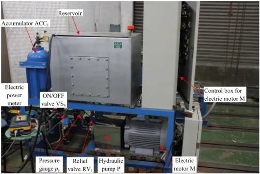
To have visual look on the FST, PMT, and SMS, some imagines of experimental systems are shown in this section as well. Figure 2.2 shows the supply response, which consists of the electric motor M, hydraulic pump P, relief valve RV1, pressure gauge ps, ON/OFF valve VS4, which acts as an unload valve,

Accumulator ACC1, and some other devices such as the reservoir and control box

for the electric motor M. Figure 2.3 shows the valve control circuits of the all three systems. For the FST and PMT systems, the valve control circuits consist three ON/OFF valves and SMS uses servo valve to control the velocity response of the ﬂywheel FW. The ﬂywheel, encoder, and hydraulic pump/motor PM are shown in Fig. 2.4.

(39)

2.1 FST System Reservoir ON/OFF valve VS4 Electric motor M Hydraulic pump P Accumulator ACC1 Relief valve RV1

Control box for electric motor M Pressure gauge ps Electric power meter

Figure 2.2: Supply response.

ON/OFF valve VS3 ON/OFF valve VS1 ON/OFF valve VS2 Relief valve RV2 Servo valve Flow meter 1 Check valve VC1 Check valve VC2

(40)

2.1 FST System Accumulator ACC2 Encoder Flywheel Hydraulic pump/motor PM Pressure gauge p3

Figure 2.4: Control valve circuit with load.

is achieved, the state of the system changes to the working phase. At this time, the control logics for the ON/OFF valves are used to regulate the velocity of the flywheel around the constant value. When the working phase is completed, the system turns to the deceleration phase. All ON/OFF valves are in a closed state; however, the pump/motor PM still works because of the kinetic energy of the flywheel FW and it acts as a hydraulic pump to convert the kinetic energy into high-pressure fluid stored in the accumulator ACC2. The pump/motor PM

is supplied with water via the suction line that contains the check valve VC2.

This energy is one part of the recovered energy; more energy is recovered in the working phase when the velocity of the ﬂywheel FW decreases.

2.1.2 Mathematical Model of Key Devices

(41)

2.1 FST System

2.1.2.1 Hydraulic Pump

The simple model of an axial piston pump is shown in Fig.2.5. Here, the pistons are arranged axially parallel to each other around the circumferential periphery of the cylinder block. The cam plate was fixed and the angle of the working surface and vertical direction is α. The pistons were connected with the shoe plate via piston shoes. When the cylinder block rotates, the position of the cylinder block and the cam plate interchanged; accordingly, the pistons are driven to and fro inside a number of bores in the cylinder barrel. Controlled by ball valves, the fluid is sucked in or pumped out, the flow rate of the pump at a given rotational speed remaining constant. However, the flow rate can vary if the speed of rotational of the prime mover is altered or the angle between the axis of the cam plate and the barrel is changed.

A A-A D d Cam plate Shoe plate Drive shaft αo Port plate Cylinder barrel Cylinder Piston A h n Outlet port Inlet port n

Figure 2.5: Model of axial piston pump.

Flow rate of the hydraulic pump can be calculated as following equation [5]:

QP = ηPAhzn (2.1)

where A is the area of piston bore and ηP is volumetric eﬃciency of the pump.

(42)

2.1 FST System

h: stroke length of the piston, h = Dtan α z: number of cylinders

n: rotational velocity of driven shaft D: diameter of the cycle of bore center α: title angle

The pump was driven by an electric motor that can be changed the rotational velocity by changing frequency of the electrical power supply via a frequency converter. Rotational velocity of electric motor can be calculated by following equation [57].

n = 120f

P (2.3)

where

n: rotational velocity of electric motor f : frequency of electrical power supply

P : number of poles for which the stator is wound

In the experimental system, the SF-JR electric motor having 4 poles and Variable Frequency Freqrol-A500 that can be changed the frequency from 0.2 to 400 Hz were used. Base on the Eq. 2.3, the rotational velocity of pump can be changed from 4 to 12000 min−1.

2.1.2.2 Relief Valve

A pressure relief valve is a normally closed valve connected between the pressure line and the reservoir. Its main purpose is to limit the pressure in a system to a prescribed maximum by diverting some or all of the pump output to the tank, when the designed pressure is reached [5]. In the FST system, two pressure relief valves were assembled. The ﬁrst relief valve (RV1) is to limit the pressure Ps in

the discharge side of the pump (P) at 12MPa that acts as supply pressure and the remaining relief valve (RV2) is to limit the pressure P1 in the line after ON/OFF

valve VS1, because pressure P1 can be reached over design pressure when the

(43)

2.1 FST System

A simple relief valve may consist of nothing but a ball or poppet held seated in the valve body by the compressive force of a heavy spring. When the pressure at the inlet is insufficient to overcome the force of the spring the valve remains closed and hence it is very often referred as a normally closed valve. When the preset pressure is reached, the ball unseats and allows flow through outlet to tank. In most of these valves, an adjusting screw is provided to vary the spring force. Thus the valve can be set to open at any pressure within the specified range. The pressure at which the valve first opens is called the cracking pressure. As the flow through the valve increases, the poppet is forced further, the resulting pressure increasing considerably thereby. The difference between the full flow pressure and the initial pressure may sometime be objectionable to other system elements. In certain cases it can result in a considerable amount of wasted power due to the fluid lost through the valve before its maximum setting is reached [5]. Figure2.6 shows a simple sketch of a pressure relief valve.

In the FST system, Nessie pressure relief valve type VRH60 which has maximum ﬂow rate of 60 l/min is used as relief valve RV2. The P/Q

characteristics of the valve shows in Fig.2.7[Danfoss Catalog] with three pressure setting ranges 10 to 40 bar, 25 to 80 bar, and alt. 80 to 140 bar. The cracking pressure of the valve was set up at 14 MPa; therefore, the P/Q characteristic of the valve corresponds to the pressure setting range 10 to 40 bar. Based on the characteristics of the relief valve type VRH60, the logic chart of the relief valve can be simpliﬁed in Fig. 2.8 with cracking pressure Pcr of 14 MPa, full ﬂow

pressure Pff of 19 MPa, and maximum ﬂow rate Qmax of 70 l/min.

2.1.2.3 Accumulator

(44)

2.1 FST System

Figure 2.6: Model of relief valve [5].

ﬂow of ﬂuid. But major disadvantage is that possibility of bladder failure which is to be taken into consideration [5]. Figure2.9 shows the component of a bladder type accumulator.

The two accumulators with diﬀerent functions are used in the system, the ﬁst one ACC1 contributed as a pressure surge absorber and the other one ACC2 is

to store the recovery energy in the pressure energy that is converted from the kinetic energy of the ﬂywheel mainly in the deceleration phase (Phase 3).

The accumulators in experiments were the bladder type. Thus, the mathematical model of a bladder type accumulator in [58] and [59] was used in this study.

(45)

2.1 FST System

Figure 2.7: P/Q characteristics of Nessie pressure relief valve type VRH60.

P Q [MPa] [l/min] P P Q cr ff max

Figure 2.8: Modeling of P/Q characteristic of relief valve.

mdu dt = dQh dt − dW dt (2.4)

where m is the mass of the gas, u the internal energy per unit mass, Q the heat energy transferring into the accumulator, and W the external work of the accumulator.

(46)

2.1 FST System

Figure 2.9: Component of a bladder type accumulator.

be calculated as follows

dQ

dt = hA(Tw− Tg) (2.5)

where h is the transfer coeﬃcient, A the heat transfer area, Tg the temperature of

the gas, and Tw the temperature of the accumulator wall. Furthermore, in fact,

the accumulators were ﬁlled with water inside so that it is necessary to consider the temperature of the water. That means the temperature of the water in the accumulators is assumed to be constant and equal to the temperature of the wall.

Moreover, the external work W can be determined by following equation dW

dt = pg dVg

dt (2.6)

where pg is the pressure of the internal gas and Vg the volume of the internal gas.

The relationship between the internal energy, the temperature and the volume of the internal gas can be expressed [58]:

(47)

2.1 FST System

where Cv is the speciﬁc heat at constant volume of the internal gas.

From Eqs. (2.4), (2.5), (2.6), and (2.7), the following expression is derived dTg dt = Tw−Tg τ − Tg mCv ( ∂pg ∂Tg ) dVg dt (2.8)

where τ is the thermal time constant of the accumulators and can be deﬁned by following equation

τ = mCv

hA (2.9)

Consider the internal gas of the accumulators as ideal gas; the equation of state of ideal gas will be applied to the internal gas as follows

pgVg = mRTg (2.10)

where R is the ideal gas constant. Equations (2.8) and (2.10) can be written down by using dimensionless quantities as follows:

dT_g∗ dt∗ = 1− T_g∗ τ∗ − K0 T_g∗ V_g∗ dV_g∗ dt∗ (2.11) p∗_gV_g∗ = T_g∗ (2.12) where K0 = R/Cv, Tg∗ = Tg/Tw, Vg∗ = Vg/V0, p∗g = pg/p0, Tg∗ = Tg/Tw, t∗ = t/τa,

and τ∗ = τ /τa; p0 is the precharge pressure and τa the thermal time constant

when all the gas was released.

Moreover, the relationship between τ∗ and V_g∗ can be expressed by following equation [58]

τ∗ = V_g∗+ 0.1 (2.13)

2.1.2.4 Solenoid ON/OFF Valve

(48)

2.1 FST System

and output port. When solenoid is at rest, it means no electric supplies to the solenoid, valve closes. When solenoid is active, it means electric supplies to the solenoid, ﬂuid from pressure chamber ﬂows through pressure relief conduit to make pressure in output port up; and then the pressure can open the diaphragm or poppet, that is the full open situation of solenoid valve.

Figure 2.10: Operation of ON/OFF Valve.

(49)

2.1 FST System

valves are 60 l/min at the pressure of 14 MPa.

Figure 2.11: Component of ON/OFF Valve.

Flow rate through the ON/OFF valves are calculated based on the orifice equation for turbulent flow. Orifices are sudden restrictions of short length (ideally zero length for a sharp-edged orifice) in the flow passage and may have a fixed or variable area [60]. Figure 2.12shows turbulent flow through an orifice. Flow rate through an orifice depends on cross sectional area of the orifice and difference of pressures in the two sides of orifice. Borrow from [61], flow rate through an orifice can be calculated as follows:

QOrifice = αdA0

√ 2

ρ∆POrifice (2.14)

where

(50)

2.1 FST System

P1 P2

d0

Orifice

Figure 2.12: Turbulent flow through an orifice.

A0: cross sectional area of oriﬁce, A0 =

πd20 4 ρ: ﬂuid density

d0: diameter of oriﬁce

∆POrifice: diﬀerence of pressures in the two sides of oriﬁce

Based on equation of flow through orifice, flow rate through ON/OFF valve can be calculated as Eq. (2.15)

QON/OFF = αdAON/OFF

√ 2

ρ∆PON/OFF (2.15)

where

AON/OFF: cross sectional area of poppet inside ON/OFF valve

∆PON/OFF: pressures diﬀerence of input/output ports of ON/OFF valve

However, it takes ﬁnite time from close state to full open state corresponding with opening area increasing from zero to maximum Amax. To simplify, it is

assumed that the increasing of opening area obeys the ﬁrst order equation as follows

AON/OFF =

Amax

T s + 1 (2.16)

(51)

2.1 FST System

Amax: opening area at the full open state

T : time constant that was deﬁned base on the real opening time of the valves

As shown in Fig. 2.13 - the characteristic of the opening area of ON/OFF valve, there are time lags for opening and closing processes, topen and tclose,

respectively. For simplification, they were approximated as the step response of a first-order system. In this research, coefficient ε will be introduced, and set up at the value of 0.02 in the opening process. That means, when the opening area got 98% of the maximum opening area, the valve was changed to the full open state directly; inversely, in the closing process, when the opening area got 2% of the maximum opening area, the valve was changed to the full close state directly. In the simulation circuit, the time lags for both the opening and closing processes were estimated from test data as shown in section 5 and had values of 40 ms and 100 ms, respectively. time Amax ε Amax tclose topen O p en in g a re a

Figure 2.13: Modeling of opening area of ON/OFF Valve.

2.1.2.5 Hydraulic Pump/motor

(52)

2.1 FST System

In this FST system, a pump/motor acted as pump or motor, depends on the situation. When high pressure fluid was supplied according to acceleration process, it acts as a motor and when no supply fluid and flywheel at high speed, it acts as a pump converting the kinetic energy of flywheel to energy as high pressure water stored into the accumulator ACC2.

Newton’s second law is applied to obtain the torque balance equation for the motor [60] IPMφ + T¨ f = 1 ηPM TPM,th− TPM,L (2.17) where

IPM: moment of inertia of the hydraulic pump/motor φ: angular of the hydraulic pump/motor shaft

TPM,L: load torque of the hydraulic pump/motor, TPM,L = IFWφ¨ ηPM: volumetric eﬃciency of the hydraulic pump/motor

The friction torque can be modeled as [60] Tf = Tvφ + sign ( ˙˙ φ) [ Tc0+ Ts0exp ( −| ˙φ| cs )] (2.18) where Tv, Tc0, Ts0, cs are coeﬃcient of friction.

Displacement volume of hydraulic motor can be deﬁned in the same way as hydraulic pump [60].

VPM,th= πd2

4 zD tan α (2.19)

The eﬀective displacement can be calculated using the estimated overall (volumetric and mechanical) eﬃciency ηPM [60]:

VPM,eff =

1 ηPM

VPM,th (2.20)

The theoretical torque is approximated by [60] TPM,th =

VPM,th

(53)

2.2 Valve Control

where ∆PHL is the pressure diﬀerence between the high-pressure line and

low-pressure line.

Moreover, the pump/motor ﬂow is determined by QPM = ηPM

VPM,th

2π φ¨ (2.22)

2.2 Valve Control

As mentioned above, the drive pattern of ﬂywheel shown in Fig. 2.14(a) consists of three phases: acceleration phase (Phase 1), constant phase (Phase 2), and deceleration phase (Phase 3). The total time for acceleration phase and working phase is twdepending on experiments. This section introduces the logic depending

on the ﬂywheel drive pattern and reference velocity of the ﬂywheel to control the ON/OFF valves (Fig.2.14 (b) and (c)). The valve VS1 is opened in both Phase 1

and Phase 2, and only closed in Phase 3. The two valves VS2 and VS3 received the

same control signal depending on ﬂywheel rotational velocity ωFW. In order to

compare the results for the FST system with/without energy recovery, the valve VS3 was opened during full cycle in without energy recovery case. In following

section, the valve switching algorithms corresponding to three phases will be introduced.

2.2.1 Acceleration Phase (Phase 1)

In this phase, the FST accelerates the ﬂywheel FW from the stationary state to a given reference rotational velocity. Once the reference is reached, the control logic switches to Phase 2. The ON/OFF valves are not controlled; they are fully opened to make water ﬂow directly from the pump P to the pump/motor PM. The electric motor M is operated at a velocity of 1200 min−1 in Phase 1.

2.2.2 Constant (Working) Phase (Phase 2)

The rotational velocity of the ﬂywheel FW between the prescribed limit ωopenand ωcloseis maintained via control logics, as shown in Fig.2.14(b). Table2.1presents

(54)

2.2 Valve Control ω_ref Phase 1 F ly w h ee l ro ta ti o n al v el o ci ty Time (a) Drive Pattern

ω_close

(b) Valve control logics with energy recovery Close Open Close Open 1 2 3 Phase 2 Phase 3

Phase 1 Phase 2 Phase 3 Phase 1 Phase 2 Phase 3

ω_open 1 2 3 1 2 3 1 2 3 1 2 3 1 3 2 1 2

(c) Valve control logics without energy recovery

3 1 2 3 1 1 2 3 2 3 ω_close ω_open tw

Figure 2.14: Control logic of ON/OFF valves.

Table 2.1: Valve operation logic in Phase 2.

Valve Open Close

VS1 Open

VS2 ωFW < 795 min−1 ωFW > 805 min−1

(55)

2.3 Energy Efficiency Improvement

velocity of the ﬂywheel exceeds ωclose, both of the ON/OFF valves VS2 and VS3

are closed to brake the ﬂywheel. Conversely, when the velocity becomes less than ωopen, the both ON/OFF valves are opened to supply energy to the hydraulic

motor M. By this control logic, the velocity of the ﬂywheel will theoretically oscillates inside the bounds ωopen and ωclose; however, the steady-state error is

larger in practice because of the eﬀect of the time delay of the experimental devices.

2.2.3 Deceleration Phase (Phase 3)

The speed of the ﬂywheel FW decelerates to zero and not that in this phase, no velocity control is performed, all the ON/OFF valves are closed. The ON/OFF valve VS3 is closed to brake the ﬂywheel and induce the energy recovery process.

The ON/OFF valve VS1 is closed to cut the supplied energy. The ON/OFF valve

VS2 is closed to keep the recovered energy inside the accumulator ACC2.

2.3 Energy Efficiency Improvement

This section introduces the original FST system,which only uses the constant velocity of the electric motor M, and the methods to reduce the energy consumption of this system.

2.3.1 Case 1 : Original FST System

(56)

2.3 Energy Efficiency Improvement

2.3.2 Case 2 : Reduced Velocity in the Electric Motor

Based on the working characteristic of a cycle, Phase 1 requires the most energy to accelerate the velocity of the ﬂywheel FW from stationary to reference velocity, Phase 2 requires less energy to maintain the ﬂywheel velocity at the reference value, and Phase 3 requires no energy. The velocity of the electric motor M was set at 1200 min−1 for the acceleration phase and 600 min−1for the working phase. These values were determined to ensure that the system would complete the full cycle for all reference velocities, particularly for the highest reference velocity of 1000 min−1, which requires the most supplied energy, and would stop in the deceleration phase.

2.3.3 Case 3 : Use of Unload Valve

The velocity of the electric motor was selected to maintain the same values for all reference velocities and established at a high value for addressing energy loss and opening the range of reference velocity. Thus, supplied energy to the system is normally higher than the requirement; one fraction is lost via relief valves and another is stored in the accumulator ACC1 and dissipated after the cycle. Thus,

using the unload valve method to limit the pressure p1.3 in a prescribed range

for all working periods is one method to reduce the energy consumption of the system. Another ON/OFF valve (VS4) was used to reduce supply pressure, ps.3,

acting as the load of supply response based on pressure p1.3. The control logic of

ON/OFF valves VS1 and VS4 is listed in Table 2.2. In this research, the bounds

of the pressure p1.3 are 8.5 and 9 MPa for p1open and p1close, respectively.

Table 2.2: Valve operation logic in Phase 2. Valve Open Close

VS1 p1.3 < p1open p1.3 ≥ p1close

(57)

2.4 Velocity Response

2.3.4 Case 4 : Use of Idling Stop Method

As in the unload valve method presented above, the idling stop method is based on the pressure p1.4 to turn the electric motor M on or oﬀ. The control logic for

ON/OFF valve VS1 and electric motor M are listed in Table2.3. The bounds of

the pressure p1.4 were also chosen at values of 8.5 and 9 MPa for p1startand p1stop,

respectively. The bounds of the pressure p1.4 were chosen as above to ensure that

the system was supplied minimal but suﬃcient energy to complete a full cycle. To ensure the homogeny for easier comparison, the same values as the bounds of the pressure p1.3 in Case 3 were chosen; however, slightly smaller values can also

be used.

Table 2.3: Valve operation logic in Phase 2. Valve (Electric motor) Open (Start) Close (Stop)

VS1 p1.4 ≤ p1start p1.4 > p1stop

M p1.4< p1start p1.4 ≥ p1stop

2.4 Velocity Response

2.4.1 Experimental Results

Table 2.4 shows the results on control performances of the rotational velocity of the ﬂywheel for the reference velocity of 600-1000 min−1. The rotational velocity percentage errors emax and emin in Phase 2 deﬁned in Eqs. (2.23) and (2.24)

decreased when the reference velocity ωref was up and did not exceeding 2.4% at

the velocity of 1000 min−1. In case that the reference velocity of the ﬂywheel is 800 min−1, the experimental results of the rotational velocity ωFW and the ﬂow

rate q2 to the accumulator ACC2 as energy recovery are shown in Figs.2.15 and 2.16, respectively.

emin =

ωref − ωmin ωref

(58)

emax=

ωmax− ωref ωref

(2.24)

Table 2.4: Control performance of rotational velocity. Reference ωmin ωmax emin emax

rotational velocity [min−1] [min−1] [%] [%]

1000 983 1024 1.70 2.40 900 882 923 2.00 2.56 800 783 823 2.13 2.88 700 681 725 2.71 3.57 600 580 625 3.33 4.17 0 10 20 30 40 0 200 400 600 800 1000 Time [s] R o ta ti o n al v el o ci ty ω F W [ m in -1 ]

with recovery without recovery

22 24 26 28 780

800 820

Magnified view

Figure 2.15: Experimental results of flywheel velocity (ωref = 800 min−1).

Furthermore, Fig.2.15 shows the velocity of the ﬂywheel with/without recovery corresponding to the ﬂywheel reference velocity of 800 min−1. With energy recovery process, the two ON/OFF valves VS2 and VS3 received the

same control signal during Phase 2 to maintain the ﬂywheel velocity around the reference velocity. When the velocity reached to the upper limit, the two valves were switched to close and the pump/motor PM acted as a pump. Consequently, the pressure p2 in the suction line of this pump/motor became lower. At the

(59)

2.4 Velocity Response 0 10 20 30 40 0 5 10 15 Time [s] F lo w r a te q 2 [ L /m in ] Phase 3

Figure 2.16: Experimental result of flow rate q2 (ωref = 800 min−1).

the discharge side of pump rose. Therefore, the big pressure difference made the flywheel velocity down rapidly. Conversely, whenever the rotational velocity of the flywheel decreased to the lower limit, the two valves were switched to open, and then the pump/motor acted as a motor.

The energy recovering was only realized in Phase 3. In case with energy recovery, all ON/OFF valves were closed during this phase. The pressure p3

became higher because the pump/motor acted as a pump. The high pressure water was stored in the accumulator ACC2 as the recovered energy after ﬂowing

through the check valve CV1 and the recovered energy would be used as another

driving source for next operation cycle. Figure 2.16 shows the ﬂow rate q2 to

ACC2 corresponding to the reference velocity of 800 min−1.

Beside, in case with no energy recovery, the control algorithms of the two ON/OFF valves VS1 and VS2 were the same as with energy recovery. However,

the valve VS3 was opened during the full cycle. The rotational velocity of the

ﬂywheel in this case is shown in Fig. 2.15. The main deference between the rotational velocities of the ﬂywheel with/without energy recovery was in the deceleration period when the valve VS2 was closed and the valve VS3 was opened.

(60)

process rapider; this implies that all of the kinetic energy of load will be dissipated in heat and/or acoustic energy.

2.4.2 Comparison of Simulated and Experimental Results

In this subsection, the comparison of the velocity errors and the energy recovery efficiency in the simulations and the experiments will be introduced. Figure2.17 shows the experimental and simulated results of the flywheel velocity at the flywheel reference velocity of 800 min−1. For more detail, Table2.5 will show the velocity percentage errors emax and emin in the simulations and the experiments.

0 10 20 30 40 0 200 400 600 800 1000 Time [s] R o ta ti o n al v el o ci ty ω F W [ m in -1 ] experiment simulation 24 25 26 27 780 800 820 Magnified view

Figure 2.17: Experimental and simulated results of flywheel velocity (ωref = 800 min−1).

Table 2.5: Control performance of rotational velocity. ωmin ωmax emin emax

[min−1] [min−1] [%] [%] Experiment 783 823 2.13 2.88

Simulation 785 820 1.88 2.5

(61)

600–1000 min−1, the experimental results were still similar to the simulated results. Therefore, it is concluded that the developed simulator has been built successfully. That makes an easy way to deﬁne the eﬀect of each component to the full system, so that the system can be renewed or developed more simply.

2.4.3 Analysis of Velocity Control Performance

One of the most important requirements of the system is to reduce the rotational velocity error of ﬂywheel in the working phase (Phase 2). In this subsection, the factors which aﬀected to the velocity error will be pointed out and methods that made the velocity error attenuate will be discussed.

Figure2.18shows the control signal of the two ON/OFF valves SV2, SV3, the

pressure p2, and the ﬂywheel rotational velocity ωFW in the event when upper

and lower limits are 805 min−1 and 795 min−1, respectively. From this ﬁgure, the characteristics of the ON/OFF valves are estimated as follows: the opening time is approximately 40 ms, corresponding to the decreasing of 6 min−1, and the maximum closing time is approximately 100 ms to the increasing of 14 min−1. These are inherently based on the characteristics of the ON/OFF valves; the hold time which avoids frequent switching signal is introduced in the valve control algorithms. At least during this hold time, each valve keeps its state. For all of three valves of the FST system, the hold time of 0.12 s was applied in the control logic. Note that, before the control signals were sent to the ON/OFF valves, they were magniﬁed via the solid state relay (SSR) devices from 5 V to 24 V. However, the time lags in the SSRs are not so big, they are only 0.5 ms and 2 ms for the opening and closing signals, respectively.

The two values of the upper and lower limit of the ﬂywheel velocity also have eﬀects on the velocity error. The two values should be chosen to guarantee that the valve open/close commands are kept more than the hold time.

(62)

2.4 Velocity Response 22 22.2 22.4 22.6 22.8 23 780 795 800 805 820 840 Time [s] R o ta ti o n al v el o ci ty ω F W [ m in -1 ]

Valve command signal

10 0 P re ss u re p2 [ M P a] ωFW p2 40ms 100ms

Figure 2.18: Pressure p2 response in experiment.

2.4.3.1 Conversion Time of Velocity Transducer

To determine the effect of the conversion time on the flywheel rotational velocity error, this study compares the results of two transducers. The first one has time constant of 63 ms, which corresponding with conversion time of 300 ms. The second device has much quick response with the conversion time of 7.6 µs.

Tables 2.6 and 2.7 show the velocity errors for the reference velocity 600–1000 min−1with the conversion time values of 300 ms and 7.6 µs, respectively. In both cases, the upper limit velocity ωclose is 810 min−1 and the lower limit

velocity ωopen is 790 min−1. The diﬀerence of the conversion time between

the two devices nearly 300 ms made the maximum velocity of the flywheel decrease 11.4 min−1 in average and the minimum velocity of the flywheel increase 13.8 min−1 in average. Consequently, reducing the conversion time is one effective way to make the rotational velocity of the flywheel in the working phase better. The comparison of the percentage error emin and emax when the FV converters

had the conversion time values of 300 ms and 7.6 µs will be shown in Figs.2.19 and 2.20, respectively. The transducer using in this research had suﬃciently quick response, the delay time was only 7.6 µs; hence, it does not need further improvement.

2.4.3.2 Threshold Velocity

(63)

Table 2.6: Velocity error of various reference velocities with conversion time of 300 ms.

Reference ωmin ωmax emin emax

1000 964 1043 3.60 4.30

900 864 941 4.00 4.56

800 761 841 5.00 5.13

700 664 740 5.14 5.71

600 561 639 6.50 6.50

Table 2.7: Velocity error of various reference velocities with conversion time of 300 ms.

Reference ωmin ωmax emin emax

1000 978 1029 2.20 2.90 900 877 928 2.56 3.11 800 778 830 2.75 3.75 700 676 730 3.43 4.29 600 574 631 4.33 5.17 5000 600 700 800 900 1000 1100 2 4 6

Reference velocity of flywheel ω

ref [min -1 ] P er ce n ta g e er ro r e m in [ % ] conversion time of 300 ms conversion time of 7.6 µs

(64)

5000 600 700 800 900 1000 1100

2 4 6

Reference velocity of flywheel ω

ref [min -1 ] P er ce n ta g e er ro r e m ax [ % ] conversion time of 300 ms conversion time of 7.6 µs

Figure 2.20: Experimental results of percentage error emax.

this FST system, the hold time of 0.12 s had to be maintained. With the same velocity transducer, the main factor which affects the hold time is to control the upper/lower deviations of the flywheel velocity. Thus, the criterion to choose the threshold velocities of the flywheel is to assure the hold time more than 0.12 s.

To evaluate the effect of the flywheel upper/lower limit velocities on accuracy of the velocity of the flywheel, following two cases of the limit velocities are considered.

Case 1 : To control the upper/lower deviations of the ﬂywheel velocity within 10 min−1. The rotational velocity of the ﬂywheel and its error for the reference velocity 600–1000 min−1 are shown in Table 2.7.

Case 2 : To control the upper/lower deviations of the ﬂywheel velocity within 5 min−1. Corresponding results to Case 1 are shown in Table 2.4.

Figure 2.18 shows the relationship of the ON/OFF valves SV2, SV3 control

signal, the pressure p2, and the ﬂywheel rotational velocity ωFW in Case 2 . It is

seen from this figure that the valve open and close commands are kept to 0.19 s and 0.25 s, respectively. This means that the hold time of the ON/OFF valves in Case 2 is satisfied. Because of larger upper limit velocity and smaller lower limit velocity in Case 1 , the period of the valve open and close commends are longer than that in Case 2 . As a result, the hold time of the ON/OFF valves in Case 1 is also satisfied.

芝浦工業大学学術リポジトリ

Improvement of Energy and Control

Performance in Water Hydraulic Transmissions

by PHAM, Ngoc Pha

Dissertation submitted to the Functional Control Systems,

Graduate School of Engineering at

Shibaura Institute of Technology

in partial fulﬁlment of the requirements for the degree of

Doctor of Engineering

Acknowledgements

Abstract

Contents

List of Figures

List of Tables

Nomenclature

Chapter 1

Introduction

1.1

Water Hydraulics

1.1.1

Historical View

1.1.2

Modern Water Hydraulics

1.1.3

Advantages and Disadvantages of Water Hydraulics

1.2

Research Objective

1.3

Outline of the Dissertation

Chapter 2

Water Hydraulic Fluid Switching

Transmission

2.1

FST System

2.1.1

Overview of the FST System

2.1.2

Mathematical Model of Key Devices

2.2

Valve Control

2.2.1

Acceleration Phase (Phase 1)

2.2.2

Constant (Working) Phase (Phase 2)

2.2.3

Deceleration Phase (Phase 3)

2.3

Energy Efficiency Improvement

2.3.1

Case 1 : Original FST System

2.3.2

Case 2 : Reduced Velocity in the Electric Motor

2.3.3

Case 3 : Use of Unload Valve

2.3.4

Case 4 : Use of Idling Stop Method

2.4

Velocity Response

2.4.1

Experimental Results

2.4.2

Comparison of Simulated and Experimental Results

2.4.3

Analysis of Velocity Control Performance