最適値関数に表れる黄金比(最適化問題における確率モデルの展開と応用)

(1)

最適値関数に表れる黄金比

(Golden

Optimal

Value

in

Discrete-time

Dynamic

Optimization

Processes)

岩本誠一

(Seiichi

IWAMOTO)

Kyushu

University,

Fukuoka

812-8581,

Japan

E-mail:

iwamoto@en.kyushu-u.ac.jp

安田正實

(Masami YASUDA)

Chiba

University,

Chiba 263-8522,

Japan

E-mail:

yasuda@math.s.chiba-u.ac.jp

概要

Aesthetics feature fascinatesmathematician. Sinceancienttimes,theGoldenRatio $(\phi)$has been

keepinngtogiveaprofound influence invariousfields. Wewill showtypical dynamic programming

problems: Allocation problem, Linear-Quadraticcontrolproblemand Multi-variatestopping prob-lem. Fortheseproblems,thereappearstheGolden Ratioin thesolution of Bellmanequation. This

paper also considers aminimization problem ofquadratic functions over an infinite horizon. We

showthat theGoldentrajectory isoptimalintheoptimization. The Goldenoptimal trajectory is

obtained through the corresponding Bellman equation, which in turn admits the Golden optimal policy. ForMulti-variatestopping problemwith three playersontheunit interval$[0,1]$, itsrelated

expectedvaluecouldbeobtainedas $\phi^{-1}$

.

KEYWORDS:

Golden Ratio, Dynamic Programming, Allocation Problem, LQ Control Problem,

Monotone StoppingProblem. Primary$90C39$; Secondary llA99.

1 lntroduction.

The Golden Ratio $(\phi=1.61803\cdots)$ has been

a

profound influence since ancient times such

as

the

ParthenonatAthens. The shape of theGoldenRatio is supposedto be interesting inagraphicformsfor

their sculptures andpaintings. The beautyappears

even

intheingredientofnature creatures. The most

influential mathematics textbook by Euclid of Alexandria defines the proportion. These information

presents

a

broad samplingof$\phi$-related topics in

an

engagingandeasy-to-understand format.

The Fibonaccisequence (1,1,2;3,5,8,13,$\cdots$ ) is closelyrelated to theGolden Ratio, whichis

a

limiting

ratioofits two adjacent numbers. It isalsoknownthat the diagonalsummation producestheFibonacci

sequence in the Pascal’striangle. These repeated procedure or iteration havesomethingin

common.

Theprinciple of Dynamic Programming is said to ‘divide and conquer.’ In fact, ifit is not poesible

(2)

original problem an effective family of sub-problems. The Bellman’s

curse

of dimensionality conquers thecomputational explosionwith the problem dimension throughthe

use

of parametricrepresentations.

The

more

it’s ina complex, the

more

it is divided. When

a

problem is in

a

multi-stage decisionform,

we

should consider the problem repeatedly. If this reduction procedure gives a self-similar one, the

methodology turns out to be effective. The Golden Ratio is created repeatedly by its

own

in a quite

same

form. A

recurrence

relationis ubiquitous. Let

us

say that

a

beautiful continued fraction represents

the Golden number. It is interesting that this quite introductory problem of Dynamic programming

produces the basic mathematlcal aspects.

In the following sections, we treat typical dynamic programming problems; Allocation problem and

Linear-Quadratic Control problem. However problems

are

in asimple fashion, it figures out the

essence

of Dynamic Programming.

Let

us

consider

a

typical type of criterion in

a

deterministic optimization. We minimize the next

quadratic criteria:

(1.1) $I(x)= \sum_{n=0}^{\infty}[x_{n}^{2}+(x_{n}-x_{n+1})^{2}]$

,

and

(1.2) $J(x)= \sum_{n=0}^{\infty}[(x_{\mathfrak{n}}-x_{n+1})^{2}+x_{n+1}^{2}]$

.

Let $R^{\infty}$ be theset ofallsequences ofrealvalues :

$R^{\infty}=\{x=(x_{0},x_{1}, \ldots,x_{n}, \ldots)|x_{n}\in R^{1}n=0,1, \ldots\}$

.

First wetake thequadratic criterion (1.1).

Nowweconsider

a

mathematical programmingproblem for anygiveninitial value $c$:

$\underline{MP_{1}(c)}$: minimize $I(x)$ subject to (i) $x\in R^{\infty}$, (ii) $x_{0}=c$

.

Let

us

evaluate

a

few special trajectories:

Example 1 First allbut

on

and$aRer$ nothing $y=\{c,$ $0,0$,

...,

$0$,

...

$\}$ yields $I(y)=2c^{2}$

.

Example 2 Always all constant $z=\{c,$ $c$

,

...,

$c$,

.. .

$\}$ yields $I(z)=\infty$

.

Example 3 A proportional (geometrical) $w=\{c,$ $\rho c$,

...,

$\rho^{n}c$,

...

$\}$ yields

$I(w)=\backslash$ $\{c^{2}+(1-\rho)^{2}c^{2}\}(1+\rho^{2}+\cdots+\rho^{2n}+\cdots)$

(13)

$=$ $\frac{1+(1-\rho)^{2}}{1-\rho^{2}}c^{2}$ $(0<\rho<1)$

.

Since

$\min_{0\leq\rho<1}\frac{1+(1-\rho)^{2}}{1-\rho^{2}}$

is attained at $\hat{\rho}=2-\phi$

,

we

have the minimum value

(3)

Example 4 The propotional $\hat{u}=\{c, (2-\phi)c, . .., (2-\phi)^{n}c, . ..\}$, with ratio $(2-\phi)$, yields

(14) $I(\hat{u})=\phi c^{2}$

.

Thus $\hat{u}=(\hat{u}_{n})$

.

gives

a

Golden optimal trajectory, because $\hat{u}_{n+1}$ is always a Golden section point of

interval $[0,\hat{u}_{n}]$

.

Next let

us now

consider

a

control process with

an

additive transition$T(x, u)=x+u$

.

minimize $\sum_{n=0}^{\infty}(x_{\mathfrak{n}}^{2}+u_{n}^{2})$

subject to (i) $x_{n+1}=x_{n}+u_{n}$, $n\geq 0$

(ii) -\infty \infty <un<o科

(iii) $x_{0}=c$

.

Then the valuefunction$v$satisfies Bellmanequation:

(1.5) $v(x)= \min_{-\infty<u<\infty}[x^{2}+u^{2}+v(x+u)]$

.

Eq. (1.5) has

a

quadratic fom$v(x)=\phi x^{2}$

.

Second

we

take the following quadraticcriterion

$J(x)= \sum_{n=0}^{\infty}[(x_{n}-x_{n+1})^{2}+x_{n+1}^{2}]$

.

Weconsider

a

problem ofform:

$\underline{MP_{2}(c):}$ minimize $J(x)$ subject to (i) $x\in R^{\infty}$, _{$(ii)x_{0}=c$}

.

Since $J(x)=I(x)-c^{2}$

,

the minimumvalue is $J(\hat{u})=(\phi-1)c^{2}$ at the Golden trajectory

$\hat{u}=\{c,$ $\mu c$,

...,

$\mu^{\mathfrak{n}}c$,

..

.

$\}$; $\mu=2-\phi$

.

In fact,

a

proportional $w=\{c,$ $\mu$,

..

.,

$\rho^{n}c$,

...

$\}$ yields

$J(w)$

$= \frac{\{\rho^{2}c^{2}+(1-\rho^{2}+(1-\rho)^{2}}{1-\rho^{2}}c^{2}(0<\rho<1)=\rho)^{2}c^{2}$

}

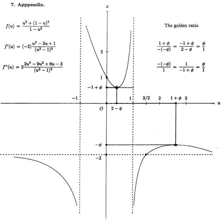
_{$(1+\rho^{2}+\cdots.+\rho^{2n}+\cdots)$}

Figure 1 in theAppendixshows that

$x^{2}+(1-x)^{2}$

$\min_{0\leq x<1}\overline{1-x^{2}}$

isattained at $\hat{x}=2-\phi$with the minimum value

(4)

2 An lllustrative Graph.

Let

us now

describe a graph which has dual Golden extremum points in the previous section. The

graph is $x=f(u)= \frac{u^{2}+(1-u)^{2}}{1-u^{2}}$ _{See Figure 1 in} _Appendix. _{For this} _function, _it _is _seen _that _two

equalities:

(2.1) $\min_{0<u<1}f(u)=\min_{0<u<1}\frac{u^{2}+(1-u)^{2}}{1-u^{2}}=-1+\phi$

and $1^{\max_{<u<\infty}f(u)}= \max_{1<u<\infty}\frac{u^{2}+(1-u)^{2}}{1-u^{2}}=-\phi$hold. Equivalently, the latter_equality_is _that

(2.2) $\min_{1<u<\infty}\{-f(u)\}=\min_{1<u<\infty}\frac{u^{2}+(1-u)^{2}}{u^{2}-1}=\phi$

The minimum in (2.1) attains iff$\hat{u}=2-\phi$, and the minimum in (2.2) attainsiff$u^{*}=1+\phi$

.

Thus

we

have the inequality

$f(u)\geq-1+\phi$

on

$(-1,1)$ and $f(u)\leq-\phi$

on

$(-\infty, -1)U(1, \infty)$

.

Refer to the shape for this graph in the Figure 1 of Appendix.

3 Dynamic Programming of

the

discrete-time

system.

The conceptualcluster of Dynamic Programmingare investigated throughout themathematics. Not only the analytical aspect ofoptimization method, but also the investigate problem with

a

repeated

structure. To give a useful explanation and

an

interesting implication,

we

show

some

explicitly solvable problems.

First the general setting of Dynamic Programming problem

are

illustrated. It is composed

as

$(S, A,r,T)$

.

Let $S$ be a state space in the Euclidean space $R$ and $A=(A_{x}),A_{x}\subset R,$$x\in S$ means

a feasible action space depending on a current state $x\in S$

.

_{The immediate reward is} a function of

$r=r(x, a,t),x\in S,$$a\in A_{x},$$t=0,1,2,$$\cdots$

.

And the terminal reward $K=K(x),$$x\in S$ is given. The

transition law fromthe current $x$ tothe new$y=m(x, a, t)$ by the action

or

decision$a\in A_{x}$ at atime$t$

.

Ifthe transition law $m(x, a, t)$ _{does not} depend $t$, it is called astationary $m(x, a,t)$ and

we

treat it in

this paper. Here

we

consider additive costs and the optimal value of $a_{t}$ will be depend on the decision

history. Assumeits value at time$t$ denoted by

$x_{t}$,which enjoythefollowing properties:

(a) The value of$x_{t}$ isobservable attime$t$

.

(b) The sequence $\{x_{t}\}$ follows

a

recurrence

in time:

(3.1) $x_{t+1}=m(x_{t}, a_{t},t)$

.

It istermed that the function$y=m(x,\pi(x,t),t)$

means a move

_{from the} current $x$to the next$y$

attsothe lawofmotion

or

the plantequation by adaptingapolicya$=\pi(x,t)$.

(5)

(d) Thecost function $C_{\pi}(x,t)$starting

a

state$x$ at time-to-go$T_{t}=T-t$ tooptimize

over

all policies

$\pi$has the additive form;

(3.2) $C_{\pi}(x_{0}, t_{0})= \sum_{t=t_{0}}^{T-1}r$($x_{t}$,at,$t$)$+K(x_{T})$

with $x_{0}=x_{t_{0}}$ and

$x_{t+1}=m(x_{t}, \pi(x_{t},t), t)$, $at=\pi(x_{t}, t)$

where$T$ is agiven finite planning horizon.

Let

$F(x,t)= \inf_{\pi}C_{\pi}(x,t)$

.

It iswellknown that the sequence $\{F(\cdot,t)\}$ satisfiesthe optimality equation(DP equation):

(3.3) $F(x, t+1)= \inf_{a\in x}[r(x,a,t)+F(m(x,a,T_{t}), t)]$

with the boundary$F(x,T)=K(x)$ where $T_{t}=T-t$ for $x\in S,$ $0\leq t<T$

.

All ofthese

are

referredfromtextbooks by Bertsekas [2], Whittle [15], Sniedovich [14], etc.

Therelationbetween TheGoldenratio formula andFibonacci sequenceis knownas [4]etc. To produce

the Fibonacci sequence, it is a good example in

a

recursive programming [13]. Also the Fibonacci

sequence

are

related with continued ffaction. Forthe notationofcontinued fraction,

we

adoptourselfto

the$follow\dot{\bm{o}}g$notations:

$b_{0}+ \frac{c_{1}}{b_{1}+\frac{c_{2}}{b_{2}+\frac{c_{3}}{b_{3}+\frac{c_{4}}{b_{4}+}}}}=b_{0}+\frac{c_{1}}{b_{1}+}\frac{c_{2}}{b_{2}+}\frac{c_{3}}{b_{3}+}\frac{c_{4}}{b_{4}+}\cdots$

.

Note that the Golden number satisfies $\phi^{2}=1+\phi$

.

By using this relation repeatedly, $\phi=1+\frac{1}{\phi}=$

$1+ \frac{1}{1+\frac{1}{\phi}}=1+\frac{1}{1+}\frac{1}{\phi}=1+\frac{1}{1+}\frac{1}{1+}\frac{1}{\phi}=1+\frac{1}{1+}\frac{1}{1+}\frac{1}{1+}\cdots$

.

Similarly the reciprocal (orsometimes called

as

a dual Goldennumber) is denoted $\phi^{-1}=0.618\cdots=\phi-1=\frac{1}{\phi}=\frac{1}{1+}\frac{1}{\phi}=\frac{1}{1+}\frac{1}{1+}\frac{1}{\phi}=\frac{1}{1+}\frac{1}{1+}\frac{1}{1+}\cdots$

This reproductive property suggestsour fundamental claim for the following typical example of

Dy-namic Programming. Beforewe solve the problem, let

us

induceasequence $\{\phi_{n}\}$ as

(3.4) $\phi_{n+1}=1+\frac{1}{1+1/\phi_{n}}=1+\frac{1}{1+}\frac{1}{\phi_{n}}$ $(n\geq 1),$ $\phi_{1}=1$

.

ノ1lso let $\{\hat{\phi}_{n}\}$

as

$\hat{\phi}_{n+1}=\frac{1}{1+}\frac{1}{1+}\hat{\phi}_{n}$ $(n\geq 1),\hat{\phi}_{1}=1$,

(3.5) i.e.

(6)

Thesequence $\{\phi_{n}\}$ of(3.4) satisfies $\phi_{n+1}$

$=1+ \frac{\frac{1}{1+1}}{1+}\frac{}{1+}\frac{\frac{1}{1+1}}{1+}\frac{i_{1}}{1+}\frac{1}{\phi_{n-2}}=1+\frac{1}{1+,1}\frac{1}{\frac\phi_{1^{n-}},1+}$

Similarly $\{\hat{\phi}_{n}\}$ of(3.5) satisfies

$\frac{1}{\hat{\phi}_{n+1}}$ $=1+ \frac{1}{1+}\frac{1}{1+}\frac{1}{1+}\hat{\phi}_{n-1}$

$=1+ \frac{1}{1+}\frac{1}{1+}\frac{1}{1+}\frac{1}{1+}n-2$

Eomthis definition, it is

seen

easily that

(3.6) $\lim_{narrow\infty}\phi_{n}=\phi=(\sqrt{5}+1)/2$

(3.7) $\lim_{n}\hat{\phi}_{n}=1/\phi=(\sqrt{5}-1)/2$

4 Linear-Quadratic

_Control

problem.

The LinearQuadratic (LQ) control problemis to minimize the quadratic cost function

over

thelinear

system. If the state of system $\{x_{t}\}$ moves on

(4.1) $x_{t+1}=x_{t}+a_{t},$ $t=0,1,2,$$\cdots$

with$x_{0}=1$ by

an

input control $\{at,$$-\infty<a_{t}<\infty\}$

.

Thecost incured 狛

(4.2) $\sum_{l=0}^{T-1}(x_{t}^{2}+a_{t}^{2})+x_{T}^{2}$

.

Then DPequation of LQ is

(4.3) $v_{t+1}(x)= \min_{a\in}\{r(a,x)+v_{t}(a+x)\}$

where

$r(a,x)=a^{2}+x^{2}$,

$a\in A_{l}=(-\infty, \infty),$$x\in(-\infty, \infty)$

Theorem 4.1 The solution of(4.3) is given by

$\{\begin{array}{l}v_{0}(x)=\phi_{T}x^{2}v_{t}(x)=\phi_{T-t}x^{2},t=1,2,\cdots\end{array}$

using the Golden numberrelated sequence$\{\phi_{n}\}$ by (3.4).

(Proof) The proofisimmediatelyobtainedby

an

elementaryquadraticminimization andthenthe

(7)

5 AIIocation

problem.

Allocationproblem or sometime called

as

partition problem,isofthe form

(5.1) $v_{t+1}(x)= \min_{a\in}\{r(a,x)+v_{t}(a)\}$

for$t=0,1,2,$$\cdots T$, where

$r(a,x)=a^{2}+(x-a)^{2}$,

$a\in A_{x}=[0,x],x\in.(-\infty, \infty)$

.

$Th\infty rem$ S.1 Thesolutionof(5.1) is given by using thedualgolden number as

$\{\begin{array}{l}v_{0}(x)=\hat{\phi}_{T}x^{2}v_{t}(x)=\hat{\phi}_{T-t}x^{2},t=1,2,\cdots\end{array}$

(Proof) Using the Schwartzinequality, the following holds immediately: Forgiven positive$\infty nstantsA$

and $B$with a fixed $x$,

$\min_{0\leq a\leq ae}\{Aa^{2}+B(x.-a)^{2}\}=\frac{x^{2}}{1/A+1/B}$

.

Sothe proofcould be done inductively. $\square$

Remark 1 : Wenoteherethat thenumber$\phi^{-1}=0.618\cdots$ ofreciprocalof the Goldennumber iscalled

sometimes Dual Golden number. The abovetwo problems

are

closely related.

Remark 2 : Itis

seen

that the

same

quadratic function of the form; $v(x)=cx^{2}$ where $c$is

a

constant,

becomes

a

solution ifthe DPequation is, for Allocation and LQ,

(5.2) $v_{t+1}(x)= \min_{a\in A_{g}}\{r(a,x)+2\int_{0}^{a}v_{t}(y)/ydy\}$

(5.3) $v_{t+1}(x)= \min_{a\in A_{*}}\{r(a, x)+2\int_{0}^{a+x}v_{t}(y)/ydy\}$

respectively. Referto [9].

6 Monotone Stopping

Game.

Amonotonerule is introducedto

sum

up individualdeclarirationsin

a

multi-variateItoppingproblem

[16]. The rule is defined by a monotone logical function and is equivalent to the winning class of

Kadane [12]. There given p-dimensional random process $\{X_{n};n=1,2, \cdots\}$ and a stopping rule $\pi$ by

which thegroup decisiondetermined from the declararion of$p$players at each stage. ThestoppIngrule

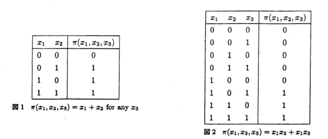
is p-variate $\{0,1\}$-valuedmonotone logical function. Weconsidertwo

cases

of rules with$p=3$

as

follows:

(6.1) $\pi(x_{1}, x_{2},x_{3})=x_{1}+x_{2}$

and

(8)

X1 $\pi(x_{1},x_{2},x_{3})=x_{1}+x_{2}$ for any$x_{3}$

$\otimes 2$ _{$\pi(x_{1},x_{2},x_{3})=x_{1}x_{2}+x_{1}x_{S}$}

Thatis, in

case

of the

case

(6.1),if either ofplayer1 and2declaresstop,then the system$stop_{8}$neglecting

of$x_{S}$

.

In

case

of (6.1),

we have

thesystem stopswheneither of player

1

and 2declaresstop accompanying

with player 1. Without loss ofgenerality,

we

can

asIumethat each $X_{n}$ takes theuniformly distribution

on

$[0,1]$

.

Then equilibrium expected values for each player is given

as

Table 1. Theequilibrium expectedvalue for each players.

Inorder to derive the value $\phi^{-1}=\frac{\sqrt{5}-1}{2}$ , wecomsider

an

equilibrium stoppingstrategy of threshold

type in the form $\{X_{n}>a\}$ for

some

$a$

.

Bellman type equationfor this gameversion will be given

as

[16].

Thatis,eachplayerdeclares “stop” or “continue” iftheobserved valueexceeds

some

$a$or not. The event

of the

occurence

is denoted by $D_{n}^{i}=$ {Player$i$ declaresstop}. Two trivial

cases are

the whole event $\Omega$

and the emptyevent $\emptyset$

.

In generally alogicalfunction is assumed “monotone” so itsfunctioncan be written

as

$\pi(x^{1}, \cdots x^{p})=x^{:}\cdot\pi(x^{1}, \cdots 1,\cdot x^{p})i..+\overline{x^{i}}\cdot\pi(x^{1}, \cdots 0,\cdot x^{p})i.$

.

$x^{:}\in\{0,1\}\forall i$

$wherex^{*}=1-x^{:}-$

.

_{Corresponding} _{to thiI}_expression,

$II(D^{1}, \cdots D^{p})=D^{i}\cdot\Pi(D^{1}, \cdots\Omega,\cdot D^{p})+\overline{D^{t}}\cdot\Pi(D^{1}:\cdot\cdot, \cdots\emptyset,\cdot\cdot D^{p})i$

.

where$\overline{D^{1}}$

is thecomplement ofthe event $D^{:}$

.

The generalequation for the expected for player $i$ at the

step $n$ equalSas follows:

(9)

where $D_{n}^{i}=\{X_{n}^{i}\geq v^{i}\}$ and $(x)^{+}= \max\{x,0\},$ $(x)^{-}= \min\{x, 0\}$. If

we assume an

independence

case

betweenplayer’s randomvariable$X_{n}^{i}$ for each $i$. The equation (6.3) becomes (6.4) $\beta_{n}^{\Pi(i)}E[(X_{n}^{i}-v^{i})^{+}]-\alpha_{n}^{\Pi(i)}E[(X_{n}^{i}-v^{i})^{-}]=0$

.

Our objective is to find

an

equilibrium strategy and values of players for

a

given monotone rule

as

the

rule (6.1) and (6.2). A sequence of expected value (a net gain) under the situation formulated in the

section isobtained

as

(6.5) $v_{n+1}^{i}=v_{n}^{1}+\beta_{n}^{II(\dot{\iota})}E[(X_{n}^{i}-v_{n}^{i})^{+}]-\alpha_{n}^{n(i)}E[(X_{n}^{i}-v_{n}^{i})^{-}]$

for player $i=1,$$\cdots$

,

$p$and$n$denotesatime-to-go. Thedetailsrefer to$Th\infty rem2.1$ inYKN [16]. Under

these derivation,

now we are

able to calculate theoptimal (equilibrium) value $v^{i}= \lim_{n}v_{n}^{1}$ for player

(10)

7. Apppendix. $x$

(11)

参考文献

[1] E.F. Beckenbachand R. Bellman, Inequalities, 3rdrevisedprinting, Springer, New York, 1971.

[2] Dimitri P. $Bertse\ovalbox{\tt\small REJECT}$

,

Dynamic Programming and Stochastic Control, Academic Press, New York,

1976.

[3] A. Beutelspacher and B. Petri, Der Goldene Schnitt 2., \"uberarbeitete und erweiterte Auflange,

El-sevier$GmbH$, Spectrum AkademischerVerlag, Heidelberg, 1996.

[4] R. A. Dunlap, The Golden Ratio andFibonacci Numbers, World Scientific Press, 1997.

[5] S. Iwamoto, InverIe theorem in dynamic programming I, II, III, J. Math. Anal. Appl. 58(1977),

113-134, 247-279, $43k448$

.

[6] S.Iwamoto, Cross dual on the Goldenoptimumsolutions, RIMSKokyuroku, Kyoto Yniv. No.1443,

pp.27-43,

2005.

[7] S.Iwamoto, Theory

_of

Dynamic Program (in Japanese), KyushuUniv. Press, Fukuoka, Japan

1987.

[8] S. Iwamoto, The Golden optimum solution in quadratic programming, Ed. W. Takahashi and T.

Tanala, Proceedings of The Fourth International Conference

on

Nonlinear Analysis and Convex

Analysis (NACA05), Okinawa, Japan, June-July, 2005, YokohamaPublishers, to aPpear.

[9] S. Iwamoto, Contrvlled integral equations

on

nondeterminstic dynamic programming: Predholm and

Volterra tyPes, Abstract ofMath Soc Japan, StatisticDivision, 51-52, March,

2003.

[10] S. Iwamoto and M. Yasuda, “Dynamic programming creates the Golden Ratio, too,” Proc.

_of

the

S白活h Intl

_Conference

on Optimization: Techniques andApplications (ICOTA 2004), Ballarat,

Au8-tralia, December

2004.

[11]

S.

Iwamoto and M. Yasuda, Golden Optimal Path in Discrete-Time Dynamic Optimization

Pro-cesses, The 15-th International Conference

on

Difference Equations and Application (ICDEA 2006),

Kyoto University, Kyoto, Japan, July, 2006.

[12] J.B.Kadane;“_{Reversibility}_of

a

MultilateralSequaentialGame: ProofofaConjectureofSakaguchi”,

J.Oper.Res.Soc.Japan,vol.21,609-516, (1978).

[13] Ron Knott, “Fibonacci Numbers and the Golden Section” in http:$//www$

.mcs.

surrey.

ac.

$uk/-$

$Personal/R.Knott/Fibonacci/f$ib. html

[14] M. Sniedovich, Dynamic Programming, Marshal Dekker, Inc. NewYork, 1992.

[15] P. Whittle, Optmization

over

Time, Dynamic Programming and Stochastic Control, Vol.$I$, John

Wiley&Sons Ltd, NewYork, 1982.

[16] M.Yasuda, J.Nakagami, M.Kurano, ““Multi-variate stopping problems with

a

monotone rule,