Incomplete Data Analysis for Economic Statistics By
Masayoshi Takahashi
経済統計のための不完全データ解析 高橋 将宜
A Dissertation submitted to
the Department of Computer and Information Science Seikei University
in partial fulfillment of the requirements for the degree of
Doctor of Science and Technology 2017
成蹊大学大学院 理工学研究科 理工学専攻情報科学コース 博士論文
Dissertation Committee:
Professor Manabu Iwasaki, Committee Chair Professor Kimio Oguchi
Professor Yukiko Nakano Professor Jinfang Wang
ii
Abstract
Incomplete Data Analysis for Economic Statistics By
Masayoshi Takahashi
Incomplete data are ubiquitous in social sciences; as a consequence, available data are inefficient and often biased. This dissertation deals with the problem of missing data in official economic statistics. Building on the practices of the United Nations Economic Commission for Europe (UNECE), the first half of the dissertation focuses on single imputation methods. After revealing that single ratio imputation is often used for economic data in the current practices of official statistics, this study unifies the three ratio imputation models under the framework of weighted least squares and proposes a novel estimation strategy for selecting a ratio imputation model based on the magnitude of heteroskedasticity. After showing that multiple imputation is suited for public-use microdata, the latter half of the dissertation focuses on multiple imputation methods. From a new perspective, this dissertation compares the three computational algorithms for multiple imputation: Data Augmentation (DA), Fully Conditional Specification (FCS), and Expectation-Maximization with Bootstrapping (EMB). It is found that EMB is a confidence proper multiple imputation algorithm without between-imputation iterations, meaning that EMB is more user-friendly than DA and FCS. Based on these findings, the current study proposes a novel application of the EMB algorithm to ratio imputation in order to create multiple ratio imputation, the new multiple imputation version of ratio imputation, providing brand-new software MrImputation implemented in R. Combining all of these findings, this dissertation will be an important addition to the literature of missing data analysis and official economic statistics.
Keywords: Missing data; multiple imputation; ratio imputation; official statistics
キーワード:欠測データ;欠損;多重代入法;比率代入法;補完;補定;公的統計
iii
Acknowledgments
I deeply appreciate Dr. Manabu Iwasaki for supervising the dissertation. In the past two years, I attended the Seikei Statistics Laboratory Seminar held by Dr. Iwasaki, where I presented all of the materials related to this dissertation. I acquired a tremendous amount of expertise on missing data analysis from Dr. Iwasaki in this seminar. Without his support and suggestions, this dissertation would never come to fruition. I also would like to thank Dr. Kimio Oguchi (Seikei University), Dr. Yukiko Nakano (Seikei University), and Dr. Jinfang Wang (Chiba University) for being the members of the dissertation committee.
The origin of this dissertation can be traced back to the Advanced Political Methodology Seminar by Dr. Valentina Bali (Michigan State University) and the ICPSR Applied Bayesian Modeling Seminar by Dr. Ryan Bakker (University of Georgia), where I first learned about multiple imputation in the context of political science research. Since then, I have been fascinated by the beauty of multiple imputation.
Part of this dissertation is related to my work at the National Statistics Center (NSTAC), an umbrella organization under the Statistics Bureau of Japan. My research at NSTAC revolved around the issue of data editing (error detection and correction) in the context of official statistics.
Special thanks go to Dr. Michiko Watanabe (Keio University) for constantly encouraging me to conduct research on imputation methods when she was NSTAC Vice-President. Also, I would like to thank Mr. Nobuyuki Sakashita (SRTI: Statistical Research and Training Institute), Mr.
Yoshiyuki Kobayashi (SRTI), Mr. Tatsuo Noro (SRTI), and Mr. Takayuki Ito (NSTAC) for exchanging ideas and thoughts on imputation methods in official statistics when we were colleagues at the National Statistics Center.
I wish to thank Dr. Shinsuke Ito (Chuo University) for inviting me to the Japan Society of Economic Statistics, where the work related to Chapter 2 was developed. Special thanks go to the participants of the UNECE Work Session on Statistical Data Editing, who responded to my surveys for Chapter 2. I also wish to thank Dr. Hiroe Tsubaki (NSTAC) for his insightful idea
iv
about ratio imputation, which helped me to complete the research related to Chapter 3. Earlier versions of Chapters 4 and 5 benefited from the feedback of Dr. Takayuki Abe (Keio University) and Dr. Tetsuto Himeno (Shiga University). Special thanks go to Mr. Yutaka Abe (NSTAC) for reviewing the mathematical proofs in the Appendix of Chapter 3 and for his valuable comments on an earlier version of Chapter 6.
The main chapters of this dissertation are based on the peer-reviewed articles that I previously published. The permission to use these articles was explicitly obtained from the publishers. I would like to thank the Japan Society of Economic Statistics for permission to use “Missing data treatments in official statistics: Imputation methods for aggregate values and public-use microdata”
(Statistics, no.112, 65-83), IOS Press for permission to use “Imputing the mean of a heteroskedastic log-normal missing variable: A unified approach to ratio imputation” (coauthored with Iwasaki, M. and Tsubaki, H., Statistical Journal of the IAOS, vol.33, no.3, in press), Ubiquity Press for permission to use “Statistical inference in missing data by MCMC and non-MCMC multiple imputation algorithms: Assessing the effects of between-imputation iterations” (Data Science Journal, in press), and JMASM Inc. for permission to use “Multiple ratio imputation by the EMB algorithm: Theory and simulation” (Journal of Modern Applied Statistical Methods, vol.16, no.1, 630-656) and “Implementing multiple ratio imputation by the EMB algorithm (R)”
(Journal of Modern Applied Statistical Methods, vol.16, no.1, 657-673).
Last but not least, my heartfelt gratitude goes to my family. My parents, Shigeyoshi and Miyuki, have always been supportive and understanding throughout the long and daunting journey to the completion of the dissertation. My grandmother, Tsuyako Tachibana, has cared about me in many respects while I grew up. My wife, Yoko, has constantly given me unwavering love that boosted the completion of this dissertation. Without their love and support, this dissertation would never become complete. I dedicate this dissertation to my family.
Table of Contents
1 Introduction ... 1
2 Imputation Methods in Official Statistics: Current and Future Perspectives ... 6
2.1 Introduction ... 6
2.2 Problems of Missing Data ... 8
2.3 Assumptions of Missing Data Mechanisms ... 9
2.4 Current Imputation Methods in Official Statistics: Deterministic Single Imputation.... 10
2.4.1 Regression Imputation ... 11
2.4.2 Ratio Imputation ... 11
2.4.3 Mean Imputation ... 12
2.4.4 Hot Deck Imputation ... 12
2.5 Current Practice of Data Editing Across the UNECE Member States ... 13
2.6 Simulation Studies on Deterministic Single Imputation Methods ... 14
2.7 Public-Use Microdata and Multiple Imputation ... 17
2.8 Multiple Imputation and Microdata Analysis ... 20
2.8.1 Regression Analysis: Missing Independent Variable ... 20
2.8.2 Regression Analysis: Missing Dependent Variable ... 22
2.9 Multiple Imputation, Microdata Analysis, and Congeniality ... 23
2.9.1 Analysis Model Subset of Imputation Model ... 23
2.9.2 Imputation Model Subset of Analysis Model ... 25
2.10 Conclusion ... 25
Appendix 2.1: Example Code of Generating and Analyzing Multiply-Imputed Data ... 26
3 A Unified Approach to Ratio Imputation for Heteroskedastic Missing Variables ... 28
3.1 Introduction ... 28
3.2 Notations and Assumptions of Missing Mechanisms ... 29
3.3 Competing Ratio Imputation Models ... 30
3.4 Unifying the Competing Ratio Estimators ... 32
3.5 Monte Carlo Evidence for Ratio Imputation Models ... 35
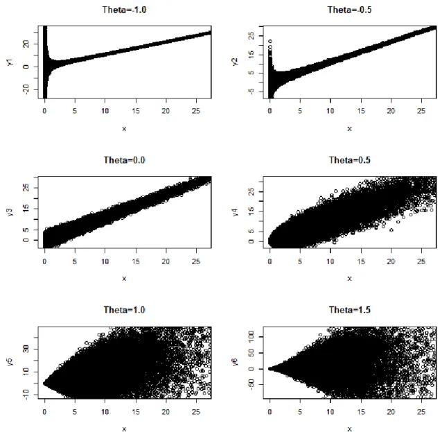
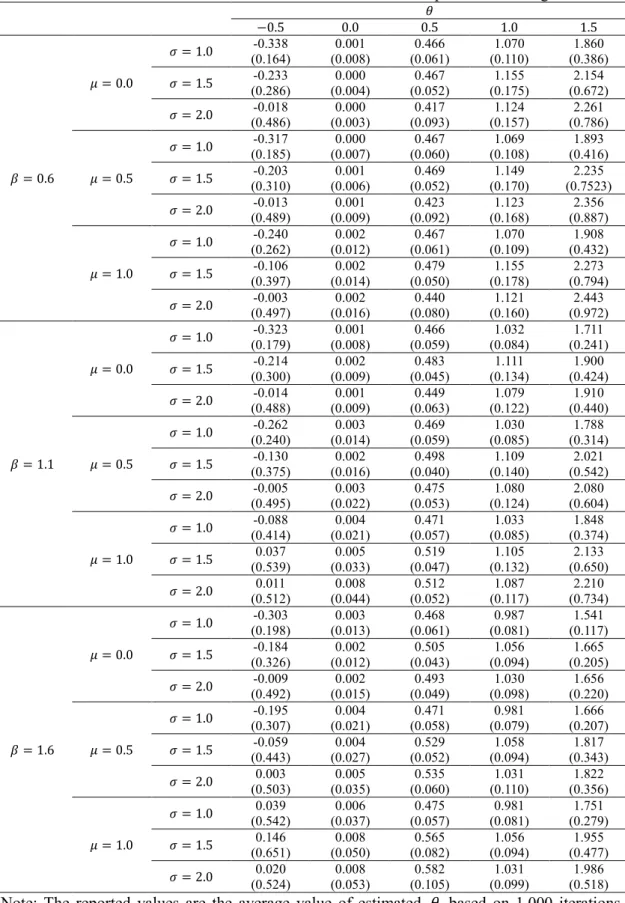
3.6 Estimating the Value of Theta... 37
3.6.1 Graphical Method of Guesstimating Theta ... 38
3.6.2 Numerical Method of Estimating Theta ... 38
3.7 Example: Application to Real Economic Data ... 43
3.8 Conclusions ... 45
Appendix 3.1 ... 46
Appendix 3.2 ... 47
Appendix 3.2.1 ... 48
Appendix 3.2.2 ... 49
Appendix 3.2.3 ... 51
Appendix 3.2.4 ... 52
Appendix 3.3 ... 53
Appendix 3.4 ... 54
4 Comparison of MCMC and Non-MCMC Multiple Imputation Algorithms ... 55
4.1 Introduction ... 55
4.2 Notations ... 56
4.3 Motivating Example: Missing Economic Data ... 56
4.4 Assumptions of Imputation Methods ... 57
4.4.1 Assumptions of Missing Data Mechanisms ... 58
4.4.2 Assumption of Ignorability ... 58
4.4.3 Assumption of Proper Imputation ... 58
4.4.4 Assumption of Congeniality ... 59
4.5 Traditional Methods of Handling Missing Data ... 59
4.6 Competing Multiple Imputation Algorithms ... 60
4.6.1 Data Augmentation ... 61
4.6.2 Fully Conditional Specification ... 62
4.6.3 Expectation-Maximization with Bootstrapping ... 63
4.6.4 Relationships among the Three Algorithms ... 64
4.7 Comparative Studies on Multiple Imputation in the Literature ... 64
4.8 Monte Carlo Simulation ... 66
4.8.1 Monte Carlo Simulation Designs ... 67
4.8.2 Criteria for Judging Simulation Results ... 69
4.8.3 Results of the Simulation: Theoretical Case ... 70
4.8.4 Results of the Simulation: Realistic Case ... 73
4.9 Conclusions ... 75
5 Multiple Ratio Imputation by the EMB Algorithm: Theory and Simulation ... 77
5.1 Introduction ... 77
5.2 Notations ... 78
5.3 Assumptions of Missing Mechanisms ... 79
5.4 Existing Algorithms and Software for Multiple Imputation ... 80
5.5 Single Ratio Imputation ... 82
5.6 Theory of Multiple Ratio Imputation ... 85
5.6.1 Nonparametric Bootstrap... 86
5.6.2 EM Algorithm ... 87
5.6.3 Application of the EMB Algorithm to Multiple Ratio Imputation ... 88
5.7 Monte Carlo Evidence ... 91
5.7.1 RRMSE Comparisons for the Mean ... 93
5.7.2 RRMSE Comparisons for the Standard Deviation ... 96
5.7.3 RRMSE Comparisons for the t-Statistics in Regression ... 98
5.8 Conclusion ... 101
6 Implementing Multiple Ratio Imputation by the EMB Algorithm in R ... 103
6.1 Introduction ... 103
6.2 Preparation Stage ... 103
6.3 Imputation Stage ... 104
6.3.1 Nonparametric Bootstrap... 104
6.3.2 EM Algorithm ... 106
6.3.3 Implementation of Multiple Ratio Imputation ... 108
6.4 Analysis Stage ... 111
6.4.1 Mean and Standard Deviation ... 111
6.4.2 Regression of y2 on y1 ... 112
6.5 Conclusion ... 113
Appendix 6.1: Software MrImputation ... 113
Appendix 6.1.1: User Manual ... 113
Appendix 6.1.2: R-Function mrimpute: Imputation Stage ... 114
Appendix 6.1.3: R-Function mranalyze: Analysis Stage ... 115
7 Conclusion ... 117
References ... 118
Curriculum Vitae ... 125
1
1 Introduction
Social science data are often incomplete, which leads to inefficient and biased analyses. This dissertation is a study of the missing data problem in official economic statistics. Specifically, this dissertation deals with single and multiple imputation methods. This chapter explains why missing data are problematic. It also shows the structure of the dissertation.
Many surveys in official statistics are based on samples because of the time and budgetary constraints. A sample is usually chosen as a subset of the population, via some type of random sampling techniques. In so doing, a random sample may be considered unit nonresponse, where some respondents do not answer in the survey, meaning that the rows for some respondents are all blank (de Waal et al., 2011, p.223). As long as sampling is random, the sampling error can be numerically assessed. Therefore, King et al. (2001, p.49) argue that unit nonresponse in social sciences generally does not introduce much bias into analyses. In fact, as the sample size increases, the law of large numbers predicts, the sampling error tends to become small (Weiss, 2005, p.329;
Ross, 2006, p.443). This may lead us to believe that, if we increase the number of observations, there will be no error in data.
A census is said to be a method to acquire information on the entire population of interest (Weiss, 2005, p.11). Once in a while, official statistical agencies have the luxury of conducting censuses in order to establish the population framework. One such example is the Economic Census for Business Activity, which aims at covering all of the enterprises and establishments in Japan. Since the census aims at obtaining information on the entire population of interest, there are no sampling errors in the census.
However, non-sampling errors and missing data occur in the measurement process of official statistics (de Waal et al., 2011, p.2). Measurement is said to be the process where numbers are assigned to objects in meaningful ways, where measurement errors occur when the attributes of empirical objects are assigned to numerical values due to the imperfect functional translation (Jacoby, 1991; Jacoby, 1999). If no numerical values are assigned to empirical objects,
2
missingness occurs due to measurement errors. In light of this, it is highly unlikely that the observations in the Economic Census will be complete. In fact, the second-term Master Plan Concerning the Development of Official Statistics (adopted by the Japanese Government in 2014) points out that it is generally difficult to obtain values for accounting items from enterprises and establishments. In other words, non-accounting items may be answered, but accounting items may not be answered by some enterprises and establishments. Although the census aims at obtaining information on the entire population of interest with no sampling error, it is likely that the census is incomplete data due to missingness.
This situation represents item nonresponse, where partial responses are available from some respondents, meaning that missing values are scattered in a data matrix (de Waal et al., 2011, p.223). To be clear about the topic of interest, this dissertation is about item nonresponse. King et al. (2001, p.49) contend that item nonresponse is more serious than unit nonresponse. In fact, whether the survey is a census or a sample does not change the fact that there are almost always some respondents who do not answer some questions in the survey. In other words, incomplete data are ubiquitous in official economic statistics, whether it is a census or a sample. When some values are missing, available data are inefficient at best and often biased at worst, without explicitly taking missing values into account. Unfortunately, this bias does not disappear when the number of observations is increased.
In light of this, the current study deals with the problem of missing data in official economic statistics, where most variables are continuous, rather than categorical. Specifically, this dissertation is a study of imputation methods, which are known to be able to rectify the missing data problem under certain assumptions. By way of organization, Chapters 2 to 6 are the body of the dissertation. Chapters 2 and 3 are mainly concerned with single imputation methods (part of Chapter 2 also with multiple imputation). Chapters 4, 5, and 6 deal with multiple imputation methods. Below is the synopsis of each chapter.
Chapter 2 reveals the status quo of official statistics around the world. For this purpose, Chapter
3
2 builds on the practices of the United Nations Economic Commission for Europe (UNECE).
Chapter 2 shows that, in the current practices of imputation among the national statistical institutes, ratio imputation is often used and indeed suitable for economic data. Also, Chapter 2 reveals that hot deck imputation is often used and indeed suitable for household data. Both of these methods are deterministic single imputation. Furthermore, Chapter 2 assesses deterministic single imputation, stochastic single imputation, and multiple imputation, demonstrating that multiple imputation is suited for public-use microdata. Therefore, this chapter indicates that the future practice of official economic statistics would need to be changed from single imputation to multiple imputation.
As is made clear in Chapter 2, ratio imputation is often used to treat missing values in official economic statistics. However, there are three competing estimators in the literature: Ordinary least squares; ratio of means; and mean of ratios. A natural question arises. Under what circumstances, which method should we use? Chapter 3 answers this question by unifying ratio imputation models under the framework of weighted least squares. Furthermore, Chapter 3 proposes a novel estimation strategy for selecting a ratio imputation model based on the magnitude of heteroskedasticity. The results in the Monte Carlo simulation give a strong support for the proposed method. This chapter should be not only academically important, but also practically useful, in choosing the best imputation method for a given dataset in an economic survey.
As Chapter 2 indicated, the future course for official statistics would be multiple imputation.
Therefore, Chapter 4 shifts gears from single imputation to multiple imputation, and compares the three computational algorithms for multiple imputation: Data Augmentation (DA), Fully Conditional Specification (FCS), and Expectation-Maximization with Bootstrapping (EMB). In the literature, many comparative studies are available from the perspectives of joint modeling (DA, EMB) and conditional modeling (FCS), which shows that joint modeling is computationally more efficient and conditional modeling is more flexible. However, little is known about the relative superiority between the MCMC algorithms (DA, FCS) and the non-MCMC algorithm
4
(EMB), where MCMC stands for Markov chain Monte Carlo. Based on simulation experiments, Chapter 4 contends that, while DA and FCS are not confidence proper without between- imputation iterations, EMB is confidence proper even without between-imputation iterations; thus, EMB is more user-friendly than DA and FCS.
Chapters 2 and 3 demonstrate that ratio imputation is often employed to deal with missing values in the practices of official economic statistics. Chapter 4 demonstrates that EMB is a useful multiple imputation algorithm. Since the literature is devoid of multiple ratio imputation, Chapter 5 proposes a novel application of the EMB algorithm to ratio imputation, so as to create the multiple imputation version of ratio imputation. Chapter 5 presents the mechanism of multiple ratio imputation and assesses the performance compared to traditional imputation methods using Monte Carlo simulation to establish the usefulness of multiple ratio imputation. Furthermore, Chapter 6 outlines a concrete code in the R statistical environment to execute multiple ratio imputation by the EMB algorithm and provides brand-new software, MrImputation implemented in R. Readers can use this software by simply copying and pasting these codes in R. Thus, this chapter should be practically useful. Finally, Chapter 7 summarizes the central findings in the dissertation and indicates the possible future courses of research. Combining all of these five chapters together, the author believes that this dissertation will be an important addition to the literature of missing data in particular and official statistics in general.
All of the chapters in the body of this dissertation are based on the peer-reviewed articles written by the author. The permission to use these articles was explicitly obtained from the publishers (See Acknowledgements). Chapter 2 is based on Takahashi (2017a), a peer-reviewed article in Statistics, which is the official journal of the Japan Society of Economic Statistics, a corporative science and research body of the Science Council of Japan. Chapter 3 is based on Takahashi et al. (2017), a peer-reviewed article in the Statistical Journal of the IAOS, which is the flagship journal of the International Association for Official Statistics (IAOS) under the umbrella of the International Statistical Institute (ISI). Chapter 4 is based on Takahashi (2017d), a peer-
5
reviewed article in the Data Science Journal, which is sponsored by CODATA (Committee on Data for Science and Technology), an interdisciplinary scientific committee of the International Council for Science (ICSU). Chapters 5 and 6 are based on Takahashi (2017b) and Takahashi (2017c), both of which are peer-reviewed articles in the Journal of Modern Applied Statistical Methods, which is operated by the Wayne State University Library System, classified as one of the top 115 libraries in the United States by the Association for Research Libraries (Kyrillidou et al., 2015). Note that the Statistical Journal of the IAOS, the Data Science Journal, and the Journal of Modern Applied Statistical Methods are indexed in Scopus by Elsevier as of April 2017.
6
2 Imputation Methods in Official Statistics: Current and Future Perspectives
This chapter derived from Takahashi (2017a), a peer-reviewed article in Statistics (112), which is the official journal of the Japan Society of Economic Statistics, a corporative science and research body of the Science Council of Japan. The author would like to thank the Japan Society of Economic Statistics for permission to use “Missing data treatments in official statistics:
Imputation methods for aggregate values and public-use microdata” (Statistics, no.112, 65-83).
2.1 Introduction
About half of the respondents generally do not answer at least one question in social surveys (King et al., 2001, p.49). Especially, the response rate tends to be low in sensitive items such as the income of individuals and the turnovers of enterprises (Schenker et al., 2006). Furthermore, respondents may unintentionally overlook or forget to answer a question. Also, if respondents change their addresses or an enterprise goes bankrupt, then values in longitudinal surveys will be inevitably missing (Allison, 2002; de Waal et al., 2011).
Thus, it is quite difficult to collect all data points in a social survey, which implies that the statistical treatment of missing values is an indispensable process in the official statistical production. While missing values in official statistics are often dealt with by imputation (de Waal et al., 2011, Ch.7), the methodological importance of imputation has rarely been discussed in Japan. On the other hand, the origin of imputation methods in official statistics can be traced back to the 1950s (U.S. Bureau of the Census, 1957, p.XXIV), which amounts to a huge body of the literature. For example, in the context of the statistical production process of microdata in official statistics, imputation methods have been the topic of debate at international conferences, such as the Work Session on Statistical Data Editing by the United Nations Economic Commission for Europe (UNECE).
In light of the findings reported at UNECE, this chapter reviews the methodological development for missing value treatments in official statistics. The first half of the chapter surveys the methods used by the UNECE member states, examining the characteristics of the imputation
7
methods for specific types of surveys such as economic surveys and household surveys in the traditional aggregation-based imputation methods.
Furthermore, while analyses were often based on macro-level data in the 20th century, it is recognized that more and more empirical analyses are based on micro-level data in the 21st century (Sakata, 2006, p.31). Under such a circumstance, there is an increasing demand that the survey data collected by official statistics should be made openly available as public-use microdata. On the supply side as well, the second-term Master Plan Concerning the Development of Official Statistics was adopted by the Japanese Government in 2014, which mentions the utilization of official statistics, where microdata will be experimentally made available at some on-site facilities (Nakamura and Hirasawa, 2016, pp.36-37). This shows that Japan has just taken a step forward in the path of public-use microdata. Thus, the latter half of the chapter discusses the future challenges about how the imputation methods for public-use microdata are different from the ones used in the traditional official statistics production process.
Note that the term “public-use microdata” in this dissertation does not imply a specific way of providing a microdata service. Unlike the traditional analysis of relying on the aggregated values tabulated by official statistical agencies, this dissertation assumes the environment where the analysts can analyze data at their discretion. In other words, the term “public-use microdata” in this dissertation refers to a larger conception that includes “public-use microdata sample,”
“anonymized microdata,” and “original data (at the individual level).” Generally, the term “public”
in this context is used for open data supplied to the general public, not for microdata supplied to the scholars who meet the terms and conditions of using microdata. However, the important point of the discussion in this chapter is that the imputers (survey organization) and the analysts (the general public and the scholars) are different entities. This chapter does not differentiate the general public and the scholars. Therefore, the term “public-use microdata” in this chapter includes the cases where the scholars are the analysts using the microdata provided by the national statistical agencies.
8
Also, note that the discussion in this chapter is limited to the topic of missing values in public- use microdata, assuming that enough level of disclosure limitation is already taken care of. For a detailed discussion on confidentiality and usability of anonymized data, see Ito and Hoshino (2014).
2.2 Problems of Missing Data
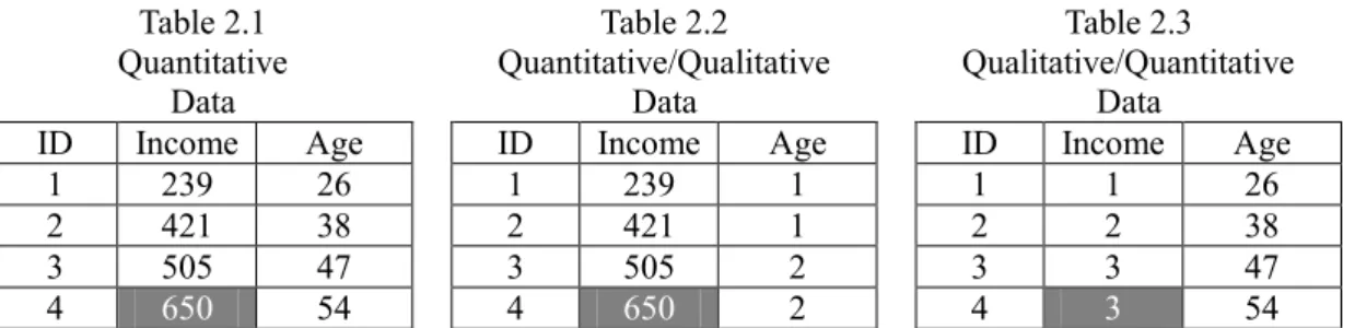
Tables 2.1, 2.2, and 2.3 are simulated data of income and age for four people. All data are continuous in Table 2.1. Age is categorical in Table 2.2. Income is categorical in Table 2.3. Black numbers are observed values, and white numbers in gray cells are the true values of the missing values. Let us assume that the estimands in Tables 2.1 and 2.2 are the mean of income, and the estimand in Table 2.3 is the mode of income.
Table 2.1 Quantitative
Data
Table 2.2 Quantitative/Qualitative
Data
Table 2.3 Qualitative/Quantitative
Data
ID Income Age ID Income Age ID Income Age
1 239 26 1 239 1 1 1 26
2 421 38 2 421 1 2 2 38
3 505 47 3 505 2 3 3 47
4 650 54 4 650 2 4 3 54
Note: The unit of income is 10,000 yen, and the unit of age is a year. In Table 2.2, 1 = less than 40 years old, 2
= 40 years or above. In Table 2.3, 1 = 0 and 2.49 million, 2 = 2.5 million and 4.99 million, 3 = 5 million or above. Tables 2.2 and 2.3 will be used in the next sections.
In Table 2.1, if all the data are observed, then the mean income of the four people can be easily calculated as 453.75 in equation (2.1).
Income
̅̅̅̅̅̅̅̅̅̅true =1
4∑ Income𝑖
4 𝑖=1
=239 + 421 + 505 + 650
4 = 453.75 (2.1)
On the other hand, as we can see in equation (2.2), even one missing value makes the calculation of the mean impossible. The fact that the mean cannot be calculated implies that the standard statistical analyses such as the computation of the standard deviation, correlation, regression coefficient, and standard error are also impossible. In other words, the primary problem of missing values is the impossibility of statistical analysis without treating missing values.
9 Income
̅̅̅̅̅̅̅̅̅̅missing=1
4∑ Income𝑖
4 𝑖=1
=239 + 421 + 505 + Income4 4
=1155 + Income4
4 =?
(2.2)
When a cell is missing in a row, then the row is deleted in the default setting of statistical software such as SAS, SPSS, and STATA. In this way, the data will be seemingly “complete,”
making statistical analysis possible. This method is called listwise deletion, also known as complete case analysis and casewise deletion (Baraldi and Enders, 2010, p.10). In Table 2.1, we treat ID4 as if it were not there; thus, the mean of income is 388.33 as in equation (2.3). However, this example shows that the true mean value is 453.75, which is underestimated due to bias in missing data. Furthermore, the valuable information about Age4= 54 is not utilized, but thrown away. The secondary problem of missing data is that the analyses based on missing data may be biased and inefficient, where bias means the difference between the expected value of the estimator and the true parameter value and efficiency means the size of variance for the estimator that becomes large as the sample size 𝑛 becomes small.
Income
̅̅̅̅̅̅̅̅̅̅listwise=1
3∑ Incomei
3 i=1
=239 + 421 + 505
3 = 388.33 (2.3)
2.3 Assumptions of Missing Data Mechanisms
Little and Rubin (2002) proposed the three classifications of missing data mechanisms: Missing Completely At Random (MCAR), Missing At Random (MAR), and Not Missing At Random (NMAR). NMAR is sometimes referred to as MNAR (Missing Not At Random), but these two are exactly the same concepts. For a more detailed discussion on the missing data mechanisms, also see Sections 3.2, 4.4, and 5.3.
Under MCAR, missing data can be considered a subsample of the population, leading to no bias, but reducing the efficiency. Under MAR, missing data may be biased. As Allison (2002, p.5) points out, we can ignore the parameters of the missing data mechanism under MCAR and MAR;
10
thus, MCAR and MAR are ignorable. As a result, imputation can rectify the bias in missing data.
On the other hand, under NMAR, the missing data mechanism is non-ignorable. The selection model and pattern-mixture model can be used to tackle the issue of non-ignorable missing data mechanisms, but these models require strong assumptions (Allison, 2002, ch.7; Enders, 2010, ch.10). As we will see later in this chapter, these methods are useful in sensitivity analysis, which evaluates how the results based on the MAR assumption would change under the assumption that NMAR is correct (Abe, 2016, p.160). If the results are not drastically different, then the confidence will be enhanced about the results based on the MAR assumption, while if the results are drastically different, then the confidence is low, so that we would need to handle the situation by including more auxiliary variables to make the assumption of MAR more relevant.
The true missing data mechanism is often unknown, but there is an occasion where the missing data mechanism is obvious through the planned missing design (Enders, 2010). For example, generally in official economic statistics, the actual turnover values among large enterprises are collected by follow-ups even if they are missing at first; then, only the missing values among small-and-medium enterprises are imputed by statistical methods (de Waal et al., 2011, pp.245- 246). In this case, the missing rate of turnover changes according to the size of enterprises such as the number of employees; thus, this can be thought of as MAR. Scheuren (2005) estimates that the proportion of MCAR is about 10% to 20%, MAR about 50%, and NMAR about 10% to 20%
in official statistics.
2.4 Current Imputation Methods in Official Statistics: Deterministic Single Imputation Traditionally, the main goal in official statistics is to compute the total (or the mean) of survey data, not the analysis of the distribution and variance (de Waal et al., 2011, p.225). Deterministic single imputation uses the predicted values based on the imputation model without adding random error. It is customary to use deterministic single imputation in official statistics, because it is an unbiased point estimator of the mean. Among the deterministic single imputation methods, it is said that the frequently used methods are regression imputation, ratio imputation, mean
11
imputation, and hot deck imputation (Hu et al., 2001; de Waal et al., 2011, ch.7). This section briefly introduces the mechanisms of these four methods.
2.4.1 Regression Imputation
In regression imputation, parameters 𝛽0 and 𝛽1 in equation (2.4) are estimated by Ordinary Least Squares (OLS) based on observed data (Takahashi et al., 2015, pp.11-14). Observed data refer to the data based on listwise deletion. Using the data in Table 2.1, we can estimate 𝛽0=
−85.33 and 𝛽1= 12.80. Since the age of ID 4 is 54, the estimated income of ID 4 is 605.87 as in equation (2.5). If we use this value instead of Income4 in equation (2.2), then the mean income is computed as 442.72. This implies that the mean value is now closer to the truth than the one based on listwise deletion. For a detailed discussion on regression imputation, also see Chapter 3 of this dissertation.
Incomê i= 𝛽0+ 𝛽1Agei (2.4) Income4= −85.33 + 12.80 × 54 = 605.87 (2.5)
2.4.2 Ratio Imputation
In ratio imputation, parameter 𝛽1 in equation (2.6) is estimated by the ratio of means based on observed data (Takahashi et al., 2015, pp.18-22). Using the data in Table 2.1, the mean of income in observed data is 388.33, and the mean of age in observed data is 37. These are the values based on listwise deletion. Therefore, we can estimate 𝛽1 = 388.33 37⁄ = 10.50. Since the age of ID 4 is 54, the estimated income of ID 4 is 567.00 as in equation (2.7). If we use this value instead of Income4 in equation (2.2), then the mean income is computed as 433.00. This implies that the mean value is now closer to the truth than the one based on listwise deletion. For a detailed discussion on ratio imputation, also see Chapter 3 of this dissertation.
Incomê i= 𝛽1Agei (2.6)
Income4= 10.50 × 54 = 567.00 (2.7)
12 2.4.3 Mean Imputation
In mean imputation, the mean of observed data is used as imputed values for missing values.
Generally, mean imputation is not useful except rare circumstances (Takahashi and Ito, 2013a, pp.27-28; Takai et al., 2016, p.6). However, in Table 2.2, the value of age is not numerical but categorical. In this situation, we may use group mean imputation, which computes the mean in each age group (de Waal et al., 2011, pp.246-249). If we stratify the data in Table 2.2 by age, then we can classify ID 1 and ID 2 to group 1, and ID 3 and ID 4 to group 2. In order to estimate the income value of ID 4, we may use the mean of group 2, which is 505. If we use this value instead of Income4 in equation (2.2), then the mean income is computed as 417.50. This implies that, unlike simple mean imputation, the mean value using group mean imputation is now closer to the truth than the one based on listwise deletion.
2.4.4 Hot Deck Imputation
Just as in Table 2.3, let us suppose that age is numeric, but income is categorical. If the estimand is categorical, we may use hot deck imputation, where we find a donor whose value in an auxiliary variable is close to that of the recipient, and the donor’s value is used as an imputation. The age of ID 4 is 54 which is close to the age 47 of ID 3 in Table 2.3. Therefore, ID 3 is the donor for ID 4. We use the income of ID 3 for the value of ID 4; thus, it will be 3. In this case, the mode of income is 3, and we can see that this value matches the true value in complete data. In the actual application, the nearest neighbor method is often used to find a suitable donor by defining the distance function, which is essentially the same as matching. For a detailed discussion on hot deck and matching, see Abe (2016, pp.57-59), Takai et al. (2016, pp.110-113), and Kurihara (2015). R Package HotDeckImputation can be used for this purpose (Joenssen, 2015). Hot deck is a non- parametric method that can be used even when all data are categorical.
13
2.5 Current Practice of Data Editing Across the UNECE Member States
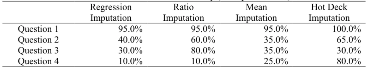
The Work Session on Statistical Data Editing is an international conference hosted every 18 months by UNECE, where national statistical agencies from Europe, North America, and Oceania meet together to exchange their ideas and information concerning the methods of handling missing values and error. The author attended the Norway conference (September, 2012), the France conference (April, 2014), and the Hungary conference (September, 2015). Questionnaires were sent to those participants who presented research papers at least in one of the above mentioned three conferences. All of them are the national statistical agencies that internationally lead official statistics. The results of the survey are summarized in Table 2.4.
Population: Twenty three national statistical agencies Survey Period: July to September, 2016
Survey Method: A questionnaire sent via email to a staff who specializes in data editing Response Rate: 87.0% (as of September 6, 2016)
Table 2.4 Results of UNECE Survey (Multiple Answers) Regression
Imputation
Ratio Imputation
Mean Imputation
Hot Deck Imputation
Question 1 95.0% 95.0% 95.0% 100.0%
Question 2 40.0% 60.0% 35.0% 65.0%
Question 3 30.0% 80.0% 35.0% 30.0%
Question 4 10.0% 10.0% 25.0% 80.0%
Question 1: Does your organization use all of the four methods in practice?
Question 2: Generally speaking, which of the four methods is most often used in practice?
Question 3: In economic data, where the unit is enterprises and establishments, which of the four methods is most often used in practice?
Question 4: In household data, which of the four methods is most often used in practice?
Question 1 reveals that all of the four methods are used in practice among almost all of the twenty national statistical agencies, where mean imputation is used more frequently than expected.
Question 2 shows that ratio imputation (60.0%) and hot deck imputation (65.0%) are deemed important. Question 3 reveals that ratio imputation (80.0%) is often used in economic data, and that regression imputation is not used very often. Incidentally, regression imputation covers a wider variety of models than ratio imputation, such as multiple regression, polynomials, logistic regression; thus, regression imputation is sometimes employed in those situations (de Waal et al.,
14
2011, pp.233-235). Question 4 shows that hot deck imputation (80.0%) is often used in household data, and that the numerical items in household data are occasionally dealt with by group mean imputation (25.0%).
Question 5 in Table 2.5 reveals the fact that, in the current practice of data editing, stochastic single imputation is used by fourteen national statistical agencies (70.0%), multiple imputation by eight national statistical agencies (40.0%), and fractional imputation by one national statistical agency (5.0%). Note that stochastic single imputation is a method that adds random components to each imputed value, so that the dispersion of data is adjusted (Takahashi et al., 2015, pp.15-18).
Table 2.5 Results of UNECE Survey (Multiple Answers) Stochastic Single
Imputation
Multiple Imputation
Fractional Imputation
Question 5 70.0% 40.0% 5.0%
Question 5: Does your organization use any of the following methods in practice? If yes, which method(s)?
This chapter does not deal with fractional imputation, but briefly, fractional imputation is a repeated imputation method just as multiple imputation. It is different from multiple imputation in the following three points (de Waal et al., 2011, p.272): (1) Fractional imputation can be considered improper multiple imputation based on the frequentist perspective; (2) the purpose of fractional imputation is to minimize the inflation of the variance in multiple imputation; and (3) fractional imputation relies on a version of hot deck; thus, it can handle qualitative data. Interested readers are referred to de Waal et al. (2011, pp.271-272).
2.6 Simulation Studies on Deterministic Single Imputation Methods
As we saw in Section 2.5, all of the four methods of mean imputation, ratio imputation, regression imputation, and hot-deck imputation are utilized by the national statistical agencies around the world. This section conducts a series of Monte Carlo simulation experiments for these four methods, assuming the following data-generation processes.
(1) Economic Data: Numerical (quantitative) data following the log-normal distribution (2) Qualitative Economic Data: Numerical (quantitative) data following the log-normal distribution and categorical (qualitative) auxiliary variable
15
(3) Household Data: Categorical (qualitative) data and numerical (quantitative) auxiliary variable
Monte Carlo simulation is an analytic method that repeatedly draws random numbers. We assume a certain probability distribution based on observed data, and generate pseudo random numbers by a computer in order to quantitatively analyze random variables that follow probability distributions (Ono and Ikawa, 2015). In other words, Monte Carlo simulation is a method to use a computer as an experimental laboratory, where the researcher has the control over the experiments and can measure the effects by observing the results based on different laboratory environments (Carsey and Harden, 2014). To be specific, Monte Carlo simulation is conducted by the following five steps (Mooney, 1997). All of the computations in Chapter 2 were done in R 3.2.4.
(1) Define the pseudo population on the computer.
(2) Draw a sample from the pseudo population.
(3) Estimate the parameter.
(4) Repeat steps (2) and (3), many times, say 1000 times.
(5) Calculate the relative frequency of the parameter estimates.
The results of the experiments are evaluated through the Mean Squared Error (MSE) in equation (2.8). The MSE of an estimate 𝜃̂ can be computed by generating a vector of true values 𝜃, taking the differences from a vector of 𝜃̂, and dividing the sum of the squared differences by the number of simulation runs (Mooney, 1997; Carsey and Harden, 2014). A smaller MSE value means that the method is comparatively good.
𝑀𝑆𝐸 = 𝐸 [(𝜃̂ − 𝜃)2] (2.8)
In the actual applications below, following Di Zio and Guarnera (2013, p.549), the Relative Root Mean Squared Error (RRMSE) is used as in equation (2.9), which normalizes the MSE by the true value and takes the square root.
16 𝑅𝑅𝑀𝑆𝐸 = √1
𝑇∑ (𝜃̂ − 𝜃 𝜃 )
𝑇 2 𝑡=1
(2.9)
The design of the simulation is as follows. The population model is equation (2.10), where the estimand is 𝑦̅.
𝑦𝑖 = 𝛽1𝑥1𝑖+ 𝜀𝑖 (2.10)
where
𝑥1𝑖~𝐿𝑁(𝑙𝑜𝑔𝑚𝑒𝑎𝑛 = 0, 𝑙𝑜𝑔𝑠𝑑 = 1) 𝜀𝑖~𝑁(𝑚𝑒𝑎𝑛 = 0, 𝑠𝑑 = 𝜎√𝑥𝑖 )
The number of iterations in Monte Carlo simulation is set to 1000, in each of which sample data with 𝑛 = 1000 are generated. The missingness in 𝑦𝑖 mimics the planned missing design (Enders, 2010) mentioned in Section 2.3. Specifically, let 𝑢𝑖~𝑈(0,1). Also, let med(𝑥1𝑖) be the median of 𝑥1𝑖. When 𝑥1𝑖< med(𝑥1𝑖) and 𝑢𝑖 < 0.6, the value of 𝑦𝑖 is made missing, which creates the MAR missingness given the values of 𝑥1𝑖. The missing rate is set to about 30%. This setting is realistic, because the mean missing rates of income and wage in the National Health Interview Survey from 1997 to 2004 are about 30%, respectively (Schenker et al., 2006, p.925).
Also, the variance of the error term 𝜀𝑖 increases in proportion to the values of 𝑥1𝑖, which means that the variance is heteroskedastic. The values of 𝛽1 are randomly drawn from 𝑈(1.1,2.0), and the values of 𝜎 are randomly drawn from 𝑈(1.0,2.0). In other runs, not reported here, where these values were changed, similar results are obtained. 𝐿𝑁(∙) is R-function rlnorm, 𝑁(∙) is R-function rnorm, and 𝑈(∙) is R-function runif, respectively.
Table 2.6 simulates the treatment of missing values in economic data, an example of which is Table 2.1. In log-normally distributed data where the variance is heteroskedastic, all of the imputation methods have smaller RRMSE compared to listwise deletion. The performance of ratio imputation (RRMSE = 0.048) is best in relation to regression imputation (RRMSE = 0.050)
17
and hot deck imputation (RRMSE = 0.050). As is discussed in Cochran (1977, p.158) and Takahashi et al. (2017), ratio imputation is the best linear unbiased estimator (BLUE) under the heteroskedastic error, 𝜀𝑖~𝑁(0, 𝜎√𝑥𝑖 ).
Table 2.6 RRMSE for Missing Value Treatments in Economic Data Complete
Data
Listwise Deletion
Regression Imputation
Ratio Imputation
Hot Deck
0.047 0.302 0.050 0.048 0.050
Table 2.7 simulates the treatment of missing values in economic data that include qualitative items, an example of which is Table 2.2. Two groups are defined by the different values of 𝑥1𝑖, 0 and 1, where the mean and the missing rate are set to different values in each group. Other settings are exactly the same as in Table 2.6. Group mean imputation (RRMSE = 0.055) outperforms listwise deletion (RRMSE = 0.081) when the auxiliary variable is qualitative.
Table 2.7 RRMSE for Missing Value Treatments in Qualitative Economic Data Complete
Data
Listwise Deletion
Mean Imputation
0.043 0.081 0.055
Table 2.8 simulates the treatment of missing values in household data that include qualitative items, an example of which is Table 2.3. The values of 𝑦𝑖 are transformed into three unordered categories, while 𝑥1𝑖 is kept numerical. The estimand is the proportion of the values that are categorized into the mode of 𝑦𝑖. Other settings are exactly the same as in Table 2.6. When the target variable for computation is qualitative, the performance of hot deck (RRMSE = 0.056) is best, and regression imputation (RRMSE = 0.381) and ratio imputation (RRMSE = 0.381) are useless in these situations.
Table 2.8 RRMSE for Missing Value Treatments in Household Data Complete
Data
Listwise Deletion
Regression Imputation
Ratio Imputation
Hot Deck
0.038 0.123 0.381 0.381 0.056
2.7 Public-Use Microdata and Multiple Imputation
Up to this point, our discussion assumes that the total (or the mean) is the target for computation.
As we saw in Section 2.5, regression imputation, ratio imputation, group mean imputation, and
18
hot deck imputation are used by the national statistical agencies around the world. As we examined in Section 2.6, these methods are used for appropriate data types. The advantage of deterministic single imputation is that it is unbiased for point estimation of the mean (or the total), but the disadvantage is that the distribution and variance are not correctly estimated (Abe, 2016, p.55). The estimand in the analysis using public-use microdata is not limited to the mean and the total.
If we want to make the analysis valid not only for the mean, but also for the variance and the standard error, we need to use multiple imputation (Schafer and Graham, 2002; Donders et al., 2006; Baraldi and Enders, 2010; Cheema, 2014). Multiple imputation, in theory, randomly draws several values from the distribution of missing data. However, missing data are unobserved; thus, the distribution of missing data is also unobserved. In real applications, we estimate the predictive posterior distribution of missing values given observed data by using Bayesian statistics, and we randomly draw the mean vector and the variance-covariance matrix from the posterior distribution.
In this way, we can implement imputation that can take into account the fact that the parameter of the imputation model is estimated (King et al., 2001). For a detailed discussion on multiple imputation, see Chapter 4 of this dissertation. Also see Iwasaki (2002, Ch.10), Takahashi and Ito (2014), Takahashi et al. (2015), and Abe (2016, Ch.5).
Table 2.9 presents a concrete example of multiply-imputed data. The empty cell in income is a missing value, and the white numbers in gray cells for income1, income2, and income3 are the imputed values by multiple imputation. The mean of income1 is estimated as 388.25, the mean of income2 as 439.75, and the mean of income3 as 475.25. The point estimate of the mean income is the mean of the three means, i.e., 428.42. Single imputation in Section 2.4 deterministically estimated one value for a missing value, seeing no estimation uncertainty. However, in Table 2.9, the imputed values change every time we impute the missing value, showing estimation uncertainty, which makes the standard error valid.
19
Table 2.9 Example of Multiply-Imputed Data (𝑀 = 3) ID Income Age Income1 Income2 Income3
1 239 26 239 239 239
2 421 38 421 421 421
3 505 47 505 505 505
4 54 388 594 664
Rubin (1987) proposes that if 𝑀 versions of multiply-imputed data (𝑀 > 1) are released by data providers, then the analysts can conduct a variety of statistical analyses regardless of their statistical literacy concerning missing data analysis. Therefore, it is suggested that multiple imputation is suitable for public-use microdata. By copying and pasting the code presented in Appendix 2.1, the analysts can perform statistical analyses without being annoyed by a practical difficulty of how to combine the analyses based on multiply-imputed data once they download public-use microdata (assuming that the public-use microdata are available online).
Table 2.10 presents concrete examples of public-use microdata provided by the U.S.
government using multiple imputation.
Table 2.10 Example of Public-Use Microdata by Multiple Imputation (U.S. Government) Organization Survey Target Variable
Number of Multiple Imputation
Publication Date Centers for
Disease Control and Prevention1
2015 National Health Interview Survey
Income, earnings 𝑀 = 5 June 30, 2016 Federal Reserve
System2
2013 Survey of Consumer Finances
Almost all missing
variables 𝑀 = 5 September 25,
2014 Department of
Transportation3
2014 Fatality Analysis
Reporting System
Blood alcohol
concentration 𝑀 = 10 December 1, 2015
Bureau of Labor Statistics4
2014 Consumer Expenditure Survey
Income 𝑀 = 5 September 3,
2015
1 http://www.cdc.gov/nchs/nhis/nhis_2015_data_release.htm
2 http://www.federalreserve.gov/econresdata/scf/scfindex.htm
3 http://www.nber.org/data/fars.html
4 http://www.bls.gov/cex/csxmicrodoc.htm
An additional survey questionnaire was sent to those twenty national statistical agencies which answered Questions 1 to 5 in Section 2.5, and the responses were obtained from eighteen agencies
20
(response rate = 90.0% as of September 6, 2016). The results are presented in Table 2.11.
Table 2.11 Results of UNECE Survey (Multiple Answers) Incomplete
Data
Deterministic Single Imputation
Stochastic Single Imputation
Multiple Imputation
None of the above
Question 6 22.0% 50.0% 61.1% 44.4% 22.2%
Question 6: Hypothetically speaking, if survey data are to be made open as “public-use microdata,” which of the following imputation methods do you think should be used?
In an open field, it was stated that public-use microdata should be imputed data so that all citizens would be able to conduct statistical analysis without being concerned with missing data.
This concurs with Rubin’s (1987) suggestion. However, consensus has not been achieved about what type of imputed data should be used, such as deterministic single imputation (50.0%), stochastic single imputation (61.1%), or multiple imputation (44.4%).
2.8 Multiple Imputation and Microdata Analysis
As we saw in Section 2.7, there is no consensus of choosing listwise deletion, deterministic single imputation, stochastic single imputation, and multiple imputation as a method to treat missing values in public-use microdata among the national statistical agencies around the world.
This section evaluates the accuracy of the mean and the regression coefficient using these four methods by Monte Carlo simulation. The number of multiply-imputed data is set to 5. This section utilizes R Package AMELIA II, a general purpose multiple imputation software program (Honaker et al., 2011). For different multiple imputation algorithms, see Chapter 4 of this dissertation.
2.8.1 Regression Analysis: Missing Independent Variable
The design of simulation is as follows (for detailed information, also see section 2.6). The population model is equation (2.11). 𝑥̅1 and 𝛽1 are the estimands. The number of Monte Carlo simulation runs 𝑇 is set to 1000, in each of which sample data of 𝑛 = 1000 are generated. The missingness in 𝑥1𝑖 is generated by MAR, conditional on 𝑦𝑖, setting the missing rate at about 30%. Specifically, just as in Section 2.6, if 𝑦𝑖 < med(𝑦𝑖), 𝑃𝑟(𝑥1𝑖 = 𝑚𝑖𝑠𝑠𝑖𝑛𝑔) = 0.6. In order to mimic the analysis based on log-normal, economic data, we assume that the data are log- transformed, so that the data were generated based on the normal distribution. The values of 𝛽1
21
are randomly drawn from 𝑈(1.1,2.0), and the values of 𝜎 are randomly drawn from 𝑈(1.0,2.0).
In other runs, not reported here, where these values were changed, similar results are obtained.
𝑦𝑖 = 𝛽1𝑥1𝑖+ 𝜀𝑖 (2.11)
where
𝑥1𝑖~𝑁(𝑚𝑒𝑎𝑛 = 0, 𝑠𝑑 = 1) 𝜀𝑖~𝑁(𝑚𝑒𝑎𝑛 = 0, 𝑠𝑑 = 𝜎)
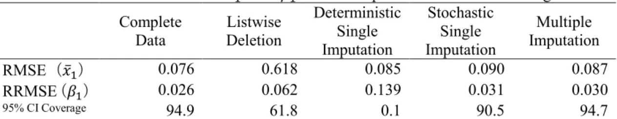
Table 2.12 shows the RMSE for 𝑥̅1, the RRMSE for 𝛽1, and the coverage rate of the nominal 95% confidence interval when missingness occurs in an independent variable.
Table 2.12 Estimation of 𝑥̅1 and 𝛽1 when Independent Variable is Missing Complete
Data
Listwise Deletion
Deterministic Single Imputation
Stochastic Single Imputation
Multiple Imputation
RMSE(𝑥̅1) 0.076 0.618 0.085 0.090 0.087
RRMSE(𝛽1) 0.026 0.062 0.139 0.031 0.030
95% CI Coverage 94.9 61.8 0.1 90.5 94.7
Note: Since the true value of 𝑥̅1 is zero, I used RMSE instead of RRMSE. CI stands for confidence interval. The 95% CI coverage means the proportion of the times the true 𝛽1 was included in the 95% confidence interval in 1,000 Monte Carlo experiments.
As for the RMSE of 𝑥̅1, both single imputation and multiple imputation are unbiased, but listwise deletion is biased. The performances of deterministic single imputation (RMSE = 0.085), multiple imputation (RMSE = 0.087), and stochastic single imputation (RMSE = 0.090) are almost equal, but the performance of listwise deletion (RMSE = 0.618) is quite low.
As for the RRMSE of 𝛽1, the performance of multiple imputation (RRMSE = 0.030) is best, followed by stochastic single imputation (RRMSE = 0.031) and listwise deletion (RRMSE = 0.062). The performance of deterministic single imputation (RRMSE = 0.139) is quite low (Allison, 2002, p.53; Carpenter and Kenward, 2013, p.28).
As for the nominal 95% confidence interval for 𝛽1, the CI by multiple imputation contains the true parameter with the probability of 94.7%, which is quite accurate. The CI by stochastic single imputation contains the true parameter with the probability of 90.5%, meaning that the nominal 5% Type I error is about double, which is a serious concern (Enders, 2010, pp.53-54). The CI by
22
listwise deletion contains the true parameter with the probability of 61.8%, meaning that the nominal 5% Type I error is about eight-fold, which is a very serious concern. The CI by deterministic single imputation contains the true parameter with the probability of 0.1%, meaning that the nominal 5% Type I error is about twenty-fold, which is an extremely serious concern.
When the independent variable has missing values and the estimands are the regression coefficient and the mean, then this analysis shows that multiple imputation should be used. Also see Chapter 4 of this dissertation about more detailed analyses, including other versions of multiple imputation.
2.8.2 Regression Analysis: Missing Dependent Variable
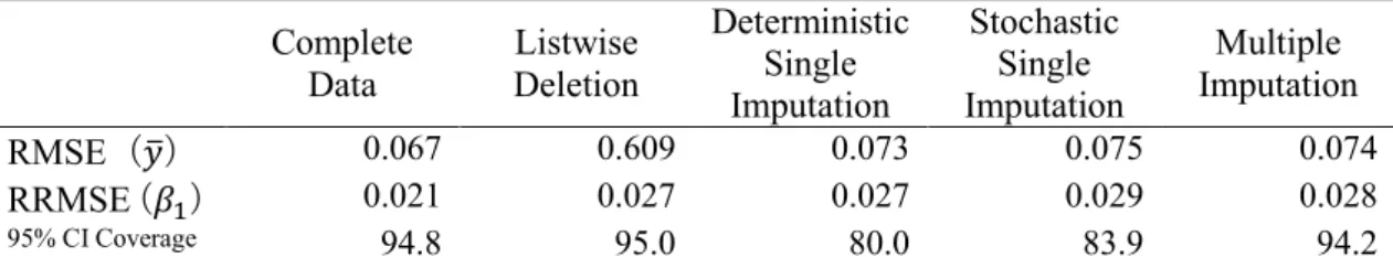
The design of simulation is as follows. The population model is equation (2.11). 𝑦̅ and 𝛽1 are the estimands. The missingness in 𝑦𝑖 is generated by MAR conditional on 𝑥1𝑖, setting the missing rate at about 30%. Other settings follow Section 2.8.1. Table 2.13 shows the RMSE for 𝑦̅, the RRMSE for 𝛽1, and the coverage rate of the nominal 95% confidence interval when missingness occurs in the dependent variable.
Table 2.13 Estimation of 𝑦̅ and 𝛽1 when Dependent Variable is Missing Complete
Data
Listwise Deletion
Deterministic Single Imputation
Stochastic Single Imputation
Multiple Imputation
RMSE(𝑦̅) 0.067 0.609 0.073 0.075 0.074
RRMSE(𝛽1) 0.021 0.027 0.027 0.029 0.028
95% CI Coverage 94.8 95.0 80.0 83.9 94.2
Note: Since the true value of 𝑦̅ is zero, I used RMSE instead of RRMSE. CI stands for confidence interval. The 95% CI coverage means the proportion of the times the true 𝛽1 was included in the 95% confidence interval in 1,000 Monte Carlo experiments.
As for the RMSE of 𝑦̅, both single imputation and multiple imputation are unbiased, but listwise deletion is biased. The performances of deterministic single imputation (RMSE = 0.073), multiple imputation (RMSE = 0.074), and stochastic single imputation (RMSE = 0.075) are almost equal, but the performance of listwise deletion (RMSE = 0.609) is quite low.
As for the RRMSE of 𝛽1, the performances of listwise deletion (RRMSE = 0.027), deterministic single imputation (RRMSE = 0.027), multiple imputation (RRMSE = 0.028), and stochastic single imputation (RRMSE = 0.029) are almost the same. When the dependent variable
23
has missing values and the estimand is the regression coefficient, then imputation does not change the result from listwise deletion. This is because the incomplete cases do not contribute to the computation of regression coefficients under MAR when missingness occurs in the dependent variable (Little, 1992; Carpenter and Kenward, 2013, pp.24-28; Raghunathan, 2016, p.99).
As for the nominal 95% confidence interval for 𝛽1, the CI by listwise deletion contains the true parameter with the probability of 95.0%, which is quite accurate. The CI by multiple imputation contains the true parameter with the probability of 94.2%, which is also quite accurate. The CI by stochastic single imputation contains the true parameter with the probability of 83.9%, meaning that the nominal 5% Type I error is more than triple, which is a serious concern. The CI by deterministic single imputation contains the true parameter with the probability of 80.0%, meaning that the nominal 5% Type I error is about quardruple, which is an extremely serious concern.
If the estimands are the regression coefficient and the mean, then multiple imputation, though it comes in second in each situation, may be the best method overall. This analysis shows that single imputation should not be used at all in this situation.
2.9 Multiple Imputation, Microdata Analysis, and Congeniality
When the imputation model and the analysis model have exactly the same variables estimating the same number of parameters, the two models are said to be congenial (Enders, 2010, p.227;
Abe, 2016, p.118; Takai et al., 2016, p.123). The models we used so far are all congenial. However, in real applications, there can be occasions under which the imputation model is different from the analysis model. If this is the case, there is no guarantee in theory about the consistency of the parameter estimates by multiple imputation. In this section, we will examine the two uncongenial cases: (1) The analysis model is the subset of the imputation model; and (2) the imputation model is the subset of the analysis model.
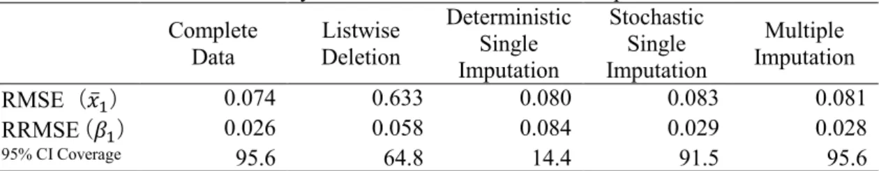
2.9.1 Analysis Model Subset of Imputation Model
The design of simulation is as follows. The imputation model is equation (2.12), and the
24
analysis model is equation (2.13). The esimands are 𝑥̅1 and 𝛽1. To be technically correct, since missingness occurs in 𝑥1𝑖, the imputation model in a strict sense is 𝑥1𝑖 = 𝛾0+ 𝛾1𝑦𝑖+ 𝛾2𝑥2𝑖+ 𝜖𝑖, and 𝑦𝑖 = 𝛽1𝑥1𝑖+ 𝛽2𝑥2𝑖+ 𝜀𝑖 is the population model of 𝑦𝑖. Equation (2.12) is equation (2.11) that contains the bivariate distribution of 𝑋. The number of Monte Carlo simulation runs 𝑇 is set to 1000, in each of which sample data of 𝑛 = 1000 are generated. The missingness in 𝑥1𝑖 is generated by MAR conditional on 𝑦𝑖, setting the missing rate at about 30%. 𝑀𝑁(∙) refers to R-function mvrnorm. The values of 𝛽1 are randomly drawn from 𝑈(1.1,1.5), and the values of 𝜎 are randomly drawn from 𝑈(1.1,1.5). In other runs, not reported here, where these values were changed, similar results are obtained.
𝑦𝑖 = 𝛽1𝑥1𝑖+ 𝛽2𝑥2𝑖+ 𝜀𝑖 (2.12)
𝑦𝑖 = 𝛽1𝑥1𝑖+ 𝜀𝑖 (2.13)
where
𝑋~𝑀𝑁(𝑚𝑒𝑎𝑛 = 0, 𝑠𝑑 = 1) 𝑋 = (𝑥1𝑖, 𝑥2𝑖) 𝑐𝑜𝑟(𝑋) = (1.0 0.60.6 1.0)
𝜀𝑖~𝑁(0, 𝜎)
When the analysis model is the subset of the imputation model, the two models are strictly speaking uncongenial. However, as is clear in Table 2.14, there is no problem in the performance of multiple imputation (Enders, 2010, pp.228-229; Carpenter and Kenward, 2013, pp.64-65).
What this implies is that the official statistical agencies as data providers can include as many auxiliary variables in the imputation model as possible, and they can make the data available after removing the variables that contain sensitive information (Takai et al., 2016, p.124). In the current practice of imputation among the national statistical agencies, the variables used for imputation are only a subset of the variables that are included in microdata; however, due to the problem of congeniality, missing values must be imputed by using all of the available variables that are
25 contained in microdata. See Section 2.9.2 below.
Table 2.14 The Analysis Model is the Subset of the Imputation Model Complete
Data
Listwise Deletion
Deterministic Single Imputation
Stochastic Single Imputation
Multiple Imputation
RMSE(𝑥̅1) 0.074 0.633 0.080 0.083 0.081
RRMSE(𝛽1) 0.026 0.058 0.084 0.029 0.028
95% CI Coverage 95.6 64.8 14.4 91.5 95.6
Note: Since the true value of 𝑥̅1 is zero, I used RMSE instead of RRMSE. CI stands for confidence interval. The 95% CI coverage means the proportion of the times the true 𝛽1 was included in the 95% confidence interval in 1,000 Monte Carlo experiments.
2.9.2 Imputation Model Subset of Analysis Model
The design of simulation is as follows. The imputation model is equation (2.14), and the analysis model is equation (2.15). Other settings follow Section 2.9.1.
𝑦𝑖 = 𝛽1𝑥1𝑖+ 𝜀𝑖 (2.14)
𝑦𝑖 = 𝛽1𝑥1𝑖+ 𝛽2𝑥2𝑖+ 𝜀𝑖 (2.15)
When the imputation model is the subset of the analysis model, as is clear in Table 2.15, the performances of all the imputation models are quite low. In other words, we should not use the analysis model that is larger than the imputation model (Enders, 2010, p.229; Carpenter and Kenward, 2013, p.64).
Table 2.15 The Imputation Model is the Subset of the Analysis Model Complete
Data
Listwise Deletion
Deterministic Single Imputation
Stochastic Single Imputation
Multiple Imputation
RMSE(𝑥̅1) 0.087 0.739 0.093 0.098 0.094
RRMSE(𝛽1) 0.036 0.063 0.119 0.117 0.115
95% CI Coverage 95.3 82.0 5.6 8.9 13.7
Note: Since the true value of 𝑥̅1 is zero, I used RMSE instead of RRMSE. CI stands for confidence interval. The 95% CI coverage means the proportion of the times the true 𝛽1 was included in the 95% confidence interval in 1,000 Monte Carlo experiments.
2.10 Conclusion
This chapter showed that the imputation methods were adopted according to the types of data in the current practice of official statistics among the UNECE member states. Specifically, ratio imputation is used for economic data, and hot deck imputation for household data. Also, the