Engineering
Copyright © 2013 by JSME
Control of Electromagnetic Current
Abstract
This paper proposes a relative position and attitude control method by using only magnetic force with multi-dipole for formation-flying spacecrafts. The control method can be widely applied to re-configurable space structures that architect large structure or reconstruct themselves by assembling basic structural units. One remarkable benefit of the method is that it does not require reaction wheels for relative attitude controls and then doesn’t require any fuel for unloading. This paper focuses on current control of dipoles which produce strong nonlinear magnetic forces and suggests a way of linearization by using a corresponding linear reference system. A feasibility of this method and controllability of the strong nonlinear system is discussed, and then the series of position and attitude control simulation are shown, and the future works are suggested in the paper.
Key words: Small Satellite, Position and Attitude Control, Formation Flight, Electro
Magnet Force, Docking
1. Introduction
One of the recent mission ideas with 10cm class small satellites such as reconfigulating the formation of some satellites to make large focal length space telescope(1) is recognized as the key technology in space field. This research proposes the way to control position and attitude of multi-bodies at a time which is especially effective in docking phase of formation flying of small satellites for restructuring its configurations to perform multi-missions. Actually there are many researches about active controls for release and docking, but most of these are for large satellites(2) or for space shuttles, and they need redundant systems to carry out their missions without fails. So the control design philosophy is totally different from the ones for small satellites, and they are not applicable in the point of mass increase and limited space. One idea to solve these problems is the use of electromagnets, but most researches of control by electromagnet are concentrating on just position control, or if any, which treats attitude control, almost all of recent research is suggesting the combination use of Reaction Wheel (RW) (3)~(11).
We point out these researches are more distant for space use in following reasons.
*
Ayako TORISAKA**, Satoru OZAWA***, Hiroshi YAMAKAWA**** and Nobuyuki KOBAYASHI**
**Aoyama Ggakuin Univ. Dept. of Mechanical Engineering, 5-10-1 Fuchinobe Chuo-Ku Sagamihara, Kanagawa,252-5258 Japan
E-mail: [email protected] ***Japan Aerospace Exploration Agency, 2-1-1 Sengen Tsukuba,Ibaraki,305-8505,Japan ****Waseda Univ. Dept. of Mechanical Engineering,
3-4-1 Okubo Shinjyuku,Tokyo,169-8555,Japan
*Received 12 Aug., 2013 (No.T2-2012-JCR-0771) Japanese Original : Trans. Jpn. Soc. Mech.
Eng., Vol.79, No.801, C (2013), pp.1540-1549 (Received 18 Oct., 2012)
at Final Docking Phase of Small Satellites
1. RW needs thruster to release its accumulated angular momentum. Using thruster means we need fuel, so this idea is fatal for permanent operation of satellites. Furthermore, thrusters take much space.
2. Other hardware use like gravity gradient or magnetorquer cannot follow frequent release of angular momentum.
Taking above mentioned points, here we suggested the use of multi-dipoles to generate torque for position and attitude control at a time. This simple mechanism doesn’t take space and mass, but enables permanent use as well, so we think our suggested control system is more reasonable than the other foregoing researches, and our idea is very new.
Here, we limit our argument in planar system for basic study with position and attitude control design, and focusing on their independent control. Then we propose our new basic control design method and report its feasibility by numerical study.
2.Attitude Control by Electro Magnet 2・1 Research target and purpose
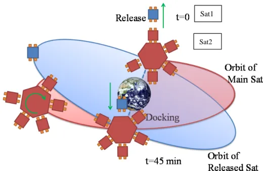
Research target is the assembled 10cm class small satellites to make space telescope by restructuring its configuration with formation flying like Fig. 1. This example shows one configulation as six small satellites are installed around a core satellite (Sat2, fixed), is going to transform into another configulation by formation flying like seven satellites are positioned in line. Generality of attitude control for docking can be kept even if we focus on any two of satellites, so we especially focused on two satellites in Fig. 2 at final docking phase, following the orbit as shown in Fig. 5 which is explained later of this setion, and supposing that the Sat2 is fixed on the original point of the coordinate because usually, the mission such as needing formation flying has a main satellite which is supposed to be a core satellite of formation flying and has a superior position and attitude controlling system, so we think the Sat2 can be treated as fixed and we want to start our arguments from this simple situation.
Our proposal is installing four dipoles on two facing surfaces of satellites each, and control their position and attitude at a time with the generated attracting force and repulsive force. Reason of four dipole use will be discussed later in this paper, and here the control force is generated by the combination of each rod’s current. In following argument, we’d like to show our proposal and satellite’s formulation in planar system as mentioned in previous chapter.
① ②
©Caltech(1)
Fig. 2 Attitude control by electro magnet
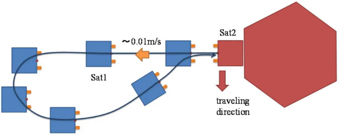
If the Sat1 was released ideally to the normal direction of its trajectory, it goes into the trajectory like coming back to the Sat2 by the inertial force produced in the orbit (Fig. 3), but here we’d like to suppose an actual release like Sat1 couldn’t follow this ideal trajectory and need some position and attitude control which follows the orbit as shown in Fig. 4 and Fig. 5. Fig. 4 shows Sat1’s requiring orbit change to going back to Sat 2 and Fig. 5 shows docking configuration in final phase when the two satellites is very close and electromagnetic force is strong enough to drive the Sat1.
Fig. 3 Satellite Orbit (ideal release) A) Orbit during the release and docking
Fig. 3 shows an orbit of two satellites when the Sat1 is released ideally in the normal direction of orbital surface like the final phase of translation ○2 to ○1 in Fig. 1. From a
broad view, this scenario shows released satellite (Sat1) is coming back to the orbit of other satellite (Sat2) 45 minuted later. However, supposing 90 min per one round in 7.5 km/s orbit and releasing Sat1 in 0.01 m/s makes orbital error of 10-5 order from exact numerical calculation by Hill’s equation, we can find the error of this order is neglectable from the following numerical calculation as well. Besides, our proposing position and attitude
dipole Sat2 Sat1
Sat2 Sat1
control method by electro magnet enables to modify this kind of trajectory error of these two satellites in final docking phase. It goes like the relative behavior of Sat1 can be corrected like Fig. 4. Also, trajectory error of satellite by the magnetic field during control is relatively very small, so we can neglect this factor, too. Additionally, another possible disturbance is solar radiation pressure, so position control is especially important and then the attitude will be also changed by this, the attitude control is required as well. Here, magnetic field by earth magnetism is smaller in double digit, the influence is negligible also.
Fig. 4 Possible Satellite Orbit B) Orbit in final phase of docking
One of the purposes of this position and attitude control in docking final phase by the multiple dipoles is moving satellites to the target state without collision, without overshoot in other words. Just using attracting force by electro magnet can’t realize this motion, so the previous researches(12),(13) using electro magnet still don’t present an approach for this prolem. From this point of view, that is to realize soft docking, we think we need to set following two phases around the vicinity of the objective position in final docking phase.
(1) Transition from Fig. 5 (a) to Fig. 5 (b) as setting Sat1 at certain distance from the objective position and make its docking surface match to y-z plane in inertia coordinate and also make the coils parallel to the coils of Sat2.
(2) Transition from Fig. 5 (b) to Fig. 5 (c) to realize simplified docking trajectory in line along x-axis only, and enhance the probability of achieving docking to the opposite face.
Here we focused on the final docking phase as the orbit like shown in Fig. 5, and set the Sat1’s target state as x b x 0 , to make our arguments simple.
(a) Initial phase (b) Pre-docking phase (c) Final phase Fig. 5 Docking configurations
Considering above, we summarized the purpose of this research as follows.
・ Suggestion of position and attitude control at a time by multiple electro -magnetic dipoles only.
・ Study about required number of dipoles.
・ Suggestion of a control row to obtain three independent control DOF (position and attitude) and its verification by numerical calculation
・ Capability for 3D formulation
2・2 Formulation of Control Force by Electro Magnet
However, originally, magnetic force is inversely proportional to the fourth power of the distance between electromagnetic moment(4), we introduced two assumptions for simplifying our arguments and formulated electromagnetic forces in planner (2D).
Assumption 1) Attraction and repulsive force by dipole are inversely proportional to square of the distance
Assumption 2) Neglect the torque by dipole, and considering just a moment by arms only.
Assumption 3) Center of the gravity of each satellite is on the middle point of two dipoles (h=0).
We formulated electromagnetic force with the model shown in Fig. 6 with additional assumption as below,
1. Set an original point of the local coordinate on the docking surface of each satellite.
2. Two dipoles are installed on each satellite, and each dipole is positioned in the distance d from the origin.
3. Neglect the sticked out distance of the dipoles. Here, Fig. 6 (b) shows only the magnetic forces from the Rod11.
(a) Sat1 (b) Magnetic force (Rod1 related) Fig. 6 Magnetic force
Regarding with disturbances such like atmospheric drag force, solar radiation pressure, gravity gradient torque, these have no relation with current I of diples, so here we treat there is control force only. Of course these disturbances can be input into f(x,I) of Eq.(1) when we do actual simulation. Further as mentioned in previous argument, we can treat Sat2 as fixed to (0,0) because we are supposing the attitude of the core satellite (Sat2) is controlled in three axis.
Equation of motion can be expressed as Eq.(1) ( , )
Mx f x I (1)
M: Mass matrix, x: position and attitude vector, I: current vector of each rod
Here, each matrix is expressed as Eq.(2) 1 1 1 1 2 1 1 1 x y m x f m y f J m h T (2)
Next, in order to generate electromagnetic forces from the two pairs of dipoles, position vector gk1,gk2 of two dipoles on each satellite are shown as Eq.(3). R(k) in Eq.(4) expresses
direction cosinevector.
1 2 1, , 2, , k k k k k k h h h h if k else if k d d d d g x R d g x R d d d d d (3) cos sin ( )= , 1, 2 sin cos k k k k k k R (4)Relative vectors between dipoles are shown in Eq.(5) and total magnetic forces are given by Eq.(6) 1 2i j 2j 1i ; ,i j1, 2 r g g (5)
11 12 1 1 11 1 1 12 ( , ) - ( ) ( ) T T T x y f f T d e d e f f f x i R f R f , 1 1 0 e (6) Here, 2 1 2 1 2 1 1121 1122 2 1 1 2 1 2 ; 1, 2 i j i j i j i j i j I I i
r f F F r r (7) ( i, i, i) . f N Const
A (8)i: magnetic permeability, Ni:Winding number, Ai:Area vector
From these equations, there is no problem even if we treat the electro magnet force as the inversely proportional to square of the distance because the basic structure of these equations are same with the actual formulation which shows the magnetic force is inversely proportional to the 4th order of the distance(4). Furthermore, although the torque from dipoles is inversely proportional to the cubic of the distance in actually, the basic structure is the distances multiply the forces in translation direction, so we can also treat this torque as the moment by the arms without a loss of generality. Regarding with mass matrix, inertia of each satellite depends on the position of its installed components, therefore our formulation with assumption 3) has no problem. Values will be offset when we do actual simulation. So the following arguments about controllability and control rows can go forward because our assumptions for simplification don’t affect to the basic structure of our proposal.
3. Attitude control by electro magnet (using linear control system to generate reference forces)
3・1 Nonlinear state equation
Shown as 2・2 , electro-magnetic force is a function of current, and it is a strong nonlinear input due to the expression as the combination product of two current. So here we tried to make this nonlinear system into the linear system by using a reference control system.
First, Eq. (1) can be rewritten into Eq. (9) as a nonlinear state equation, here f is a function of I(t).
( ) ( , ) , , T h g X AX Bf X X I X x x (9) 1 , , is unit matrix 0 eye 0 A B eye 0 0 M (10)3・2 Linearization of nonlinear system using reference system
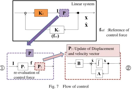
Fig.7 shows a linear control system to the Plant. Current I can be obtained by using Eq. (18) which is mentioned later (K2). To obtain the current, we need reference control force, so the point of our proposal is preparing an appropriate (= controllable) reference control system from which we can obtain its control force by giving appropriate gain K1, and set the force as fref.
Here we explain the contents of K2in Fig.7, which shows how to linearize the nonlinear dynamic system in equations.
P K2 K1
x
x
P2 P1 I f P B A∫
x x P2:Update of Displacementand velocity vector
(fref) fref :Reference of control force Linear system I re-evaluation of control force
Fig. 7 Flow of control
Defining the control force in Eq. (1) as the summation of stiffness matrix and damping matrix for linearization can obtain the Eq. (11)
2 12 1 1
x ζωx ω x 0
(11)
Then reference control force fref can be obtained as Eq.(12) by designing the dynamics of this linear system with appropriate parameters and in this linearization method.
2 1 1 (2 ) ref f M ζωx ω x (12)
1 2 11 21 11 22 12 21 12 22 T T x y f f T I I I I I I I I f D D (13)②
①
On the other hand, Eq. (3) which express the control force can be rewritten as Eq. (13). Here each current can be decided from Eq.(11),(13)-(15). The term of multiplied current is rewritten as Eq. (16) and when we put E1 = [a1 a2 a3] T,Ε2= I12 I21 = a2 a3 / a1 = t ( = function of E1),Eq.(13) can be rewritten as Eq.(17).
1 2 11 12 21 22 3 T a a I I I I a t (16) 1 1 2 2 f D E D E (17)Next, a1 ~ a3 can be decided from Eq. (18) by obtaining E1 to satisfy fref = f(E1). So E1 can be expressed by using inverse function as Eq. (18), and then each current can be obtained from Eq. (19) by using obtained E1
1 1 f E f (18) 11 2/ 22, 12 2 3/ ( 1 22), 21 1 22/ 2 I a I I a a a I I a I a (19)Here, taking notice that one of the four input Iij comes to be dependent variable, so we need to introduce some kind of constraints condition such like the minimization of current energy as min (I112 + I122 + I132 + I142). Then we can decide all of current value from
2 2 2 2 2
4
22 2 3/ 11 / 1/ 21
I a a a a a and Eq. (19). Consequently current design, control forces in
other words, can be designed with this calculation sequence in each time. Addition to above points, its another benefit that one of the current values don’t stick out because the four current have symmetric property.
Above is the detail of K2 in Fig. 7, and this linearization of nonlinear system by using a reference system.
3・3 Relation of control DOF and input current
Regarding with control DOF, the remarkable point of this system is that even the total number of dipole is four and having four control input, one of them becomes independent of other three as mentioned in 3・2 because control forces are decided by combinations of current product. Hence, it is an important knowledge that we need four dipoles to obtain
1121 1122 1221 3 3 3 1121 1122 1221 1121 1122 1221 1 3 3 3 1121 1122 1221 1121 1122 1221 1 1 3 1 1 3 1 1 3 1121 1122 1221 - ( ) - ( ) ( ) x x x y y y T T T d e d e d e r r r r r r r r r D r r r r r r R R R r r r (14)
1222 3 1222 1222 2 3 1222 1222 1 1 3 1222 ( ) x y T d e r r r D r r R r (15)dependant control forces in three axis as translation and rotation of planar system. However, fundamentary, three dipoles in total are enough in geometrical constraint viewpoint and also enough from control DOF aspect, it becames 2 DOF control in one translation and one rotation. This system is not impossible to control toward objective position, but control row becomes more complicated. Further, considering that sensitive three dependent DOF control will be needed in final docking phase like Fig. 5 (c), so installing four dipoles has more advantage which enables to handle more DOF.
4. Parameters for Numerical Calculation
Here we focused on the transition of Sat1 as from Fig. 5(a) to (b), and showed the numerical verification of our proposal as controlling the Sat1 from the initial state x1=[-1,-0.2,/60]T,
1
x =[0,0,0]T
to the final state x1 =[0,0,0]T,x =[0,0,0]1 T
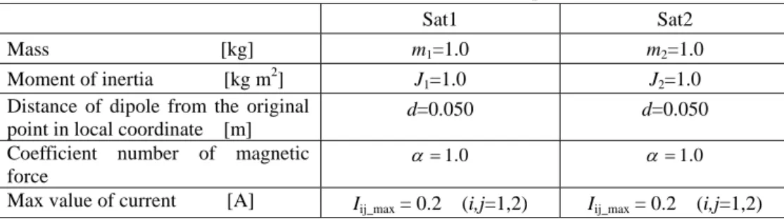
. Sat2 was set as fix x2 [0,0,0]T,x2 = [0,0,0]T, and Table 1 shows parameters of satellites and dipoles. Here, =1.0, =1.0, and simulated with the time span t = 0.0~10.0[s]. This assumption of 1m distance apart of two satellite is much far than actual situation as about 10cm use. Usually,when two satellites are far, the core satellite which has superior control system is going to come close of the daughter sateliite within their controllable region, here we wanted show our proposing method can be usable in much far region that ensure its reliability, too. and are dicided as the bevavior of the satellite becomes critical damping. Regarding with the current limit, upper or lower limit value was adopted when the calculated current was over the limited value. is constant and a function of the winding number and magnetic permeability as shown in Eq.(8).
Table 1 Parameters of satellites and dipoles
Sat1 Sat2
Mass [kg] m1=1.0 m2=1.0
Moment of inertia [kg m2] J1=1.0 J2=1.0
Distance of dipole from the original point in local coordinate [m]
d=0.050 d=0.050
Coefficient number of magnetic force
1.0
1.0
Max value of current [A] Iij_max = 0.2 (i,j=1,2) Iij_max = 0.2 (i,j=1,2)
5.Results
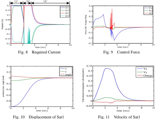
Fig. 8 to Fig. 11 shows the simulation results. Time history of each dipole’s current as control unput are shown in Fig. 8, time history of control force after linearization of whole system are shown in Fig. 9, position and attitude are shown in Fig. 10, velocity and angular velocity are shown in Fig. 11 respectively.
Focusing on Fig. 8 , we could obtain three phase of current design as follows. ① 0~2.0[s] : Mainly generating control force to start moving Sat1 in x-axis
direction.
② 2.0~3.3[s] : Mainly generating minus directioned force to slow down the Sat1 which would be a disturbance to the rotation motion at the same time. Also this behavior can be seen from Fig. 11 which shows acceleration is changing from positive to negative in a slow pace.
③ 3.3~10.0[s] : Control force is converged into 0 in all axis without overshooting, and position and attitude were also converged into our target value. The values of each current were different between Sat1 and Sat2. So we can find the position and attitude control by multi-dipole was effectively worked out between the two satellites.
Spikes in 2.8~3.2[s] of Fig. 8 are caused by the event of generating brake forces at 2.2[s] in x-axis that mean the sign of acceleration come to be opposite. This event causes the change of velocities, then reference forces come to be vibrationally, so the spikes appears. Although this problem always appears our control system as far as it requires brake phase, we think this spikes is not a fatal because these are on a certain envelope and essentially doesn’t diverge. A problem is just that our calculation in Eq.(18) couldn’t find the exact value on the envelope because of numerical approach. However, appropriate choice of a numerical method or frequent switch of control row would be a solution of this problem, we didn’t consider them in this paper for the purpose of showing the feasibility of our proposing control system as simply as possible.
Fig. 8 Required Current Fig. 9 Control Force
Fig. 10 Displacement of Sat1 Fig. 11 Velocity of Sat1
From above, we could verify and demonstrate that our proposing method of using multi-dipoles and linearization method by using reference controllable system, can simultaneously control the position and attitude of two bodies. Additionally this can be realized only by electromagnets.
6. Discussion
From the view point of required number of dipoles for expanding our arguments into spatial coordinate system, so the required control DOF is six in this case. Although three dipoles for each satellite (six in total) is enough for geometrical constraints, the independent input DOF becomes five in this case, so the one dipole comes to be dependent of others. Therefore, considering symmetric property, four dipole for each satellite is reasonable to obtain six (or more) dependent control DOF. One becomes redundant in this case, but it’s easy to put this parameter into constraints condition such like minimizing total energy or so. Further, our proposal story doesn’t have fatal effect to 3D expansion, so we believe our proposal can be effective in 3D argument also.
When deciding current value in Eq. (18), this may turn to be singular when Sat 2 is on the x axis and parallel with Sat1 and then its controllability degrades. In spite of the degradation,
0 2 4 6 8 10 -0.2 -0.15 -0.1 -0.05 0 0.05 0.1 0.15 0.2 time [sec] Am p ai r [ A] I11 I12 I21 I22 0 2 4 6 8 10 -0.3 -0.2 -0.1 0 0.1 0.2 0.3 0.4 time [sec] F o rc e [N ] / T o rq u e [N m ] Fx Fy M 0 2 4 6 8 10 -1 -0.8 -0.6 -0.4 -0.2 0 0.2 0.4 time [sec] pos it ion [ m ] / a n gl e [ ra d] x y angle 0 2 4 6 8 10 -0.05 0 0.05 0.1 0.15 0.2 0.25 0.3 0.35 time [sec] V elo city[ m /s ]/ an gula r ve lo city[ ra d/s ] Vx Vy Omega ① ② ③
this is practically not a problem because Sat2 is passing through the x axis instantaneously when Sat2 is moving. Even in the exceptional case that the Sat2 is parallel with Sat1 and moving along the x axis, the control problem becomes an only distance control problem and Sat2 is controllable by changing a simpler controller that does not includes the angle (attitude) control.
Regarding with the input, saturation of input may cause the deterioration of control performance or instability of the system, so we think we need to work on introducing another method which enables to consider input limit or saturation like Anti-windup control as our future works. One more is about actual control force. It is inversely proportional to the 4th power of the distance between two satellites that makes the formulation as strong non-linear one. So we think we need to introduce optimum control into this non-linear problem to minimize the error of linearization to the reference system, and using our proposal of this time as an initial guess, or it’s possible to choose non-linear system as a reference system as far as it is controllable.
Still there are some future works like anove, the point we want to say in this paper is that we could show the feasibility of new control method by using multi-dipole which can control position and attitude at a time and enable to be used eternally.
7. Summary
We proposed a new method of using multi-dipoles on final docking phase of small satellites to control their position and attitude at a time. This idea can be applied to a basic technology of restructuring module structures for architecting a large space structure because of the possibility of its eternal use. Further, we carried out a basic study of control row and obtained following results.
・ We suggested a way of linearization of the nonlinear system by using a controllable reference system and studied the controllability of obtained control row.
・ Feasibility of our proposal that can obtain independent control forces of three axis, was verified in planar coordinate system, and showed that our proposal is applicable into spatial coordinate system also.
・ Required numbers of dipoles in planar and spatial coordinate system are discussed. Considering symmetric property, four rods for planar coordinate and eight rods for spatial coordinate system is needed to obtain independent control DOF.
Acknowledgement
Part of this study is supported by "Institutional Program for Young Researcher Overseas Visits, JSPS", and we thank to the AAReST project members of California In stitute of Technology for helpful advicement and research information.
References
(1) Keith, P., and Sergio, P., “Shape Correction of Thin Mirrors”, Proceeding of 52nd
AIAA/ASME/ASCE/AHS/ASC Structures, Structural Dynamics and Materials Conference
(2011) , AIAA 2011-1827.
(2) Isao,K., et.al, “Result of Rendezvous Docking Experiment of ETSVII”,Journal of the Japan Society for Aeronautical and Space Sciences, Vol. 50, No. 578 (2002) , pp. 95-102. (3) Ping, Wang., and Yuri B. S., “Satellite Attitude Control Using Only Magnetictorquers” ,
Proceeding of AIAA Guidance Navigation and Control Conference and Exhibit(1998) ,
AIAA-98-4430.
(4) Ryosuke, K., Shin-ichiro, S., Tatsuaki, H., amd Hirobumi, S., “The relative position control in formation flying satellites using super-conducting magnets” , Journal of the Japan
(5) Edmund, M.C.K.., Daniel W.K.., Samuel, A.S., Laila, M.E., Raymond, J. S., and David W. M., “Electromagnetic Flight for Multisatellite Arrays”, Journal of spacecraft and Rockets, Vol.41, No.4(2004), pp. 659-666.
(6) Samuel, A.S., and Raymond J.S., “Explicit Dipole Trajectory Solution for Electromagnetically Controlled Spacecraft Clusters”, Journal of Guidance Control and
Dynamics, Vol.33, No.4(2010), pp. 1225-1235.
(7) Elias, L.M., Kwon, D.W., Raymond J.S., and Miller, D.W., “Electromagnetic Formation Flight Dynamics including Reaction Wheel Gyroscopic Stiffening Effects”, Journal of
Guidance Control and Dynamics, Vol. 30, No. 2(2007), pp. 499-511.
(8) Daniel, W.K., Raymond, J.S., Sang-il, L., Jaime L.R.R., “Electromagnetic Formation Flight test bed Using Superconducting Coils”, Journal of Spacecraft and Rockets, Vol. 48, No. 1(2011), pp. 124-134.
(9) Rafal, W., “Satellite Attitude Control Using Only Electromagnetic Actuation”, Ph.D. Thesis
Aalborg Univ, Dec (1996) .
(10) Marco, L., Alessandro, A., “Global Magnetic Attitude Control of Spacecraft in the Presence of Gravity Gradient”, IEEE Transactions on Aerospace and Electronic Systems, Vol.42, No.3(2006), pp.796 - 805.
(11) Umair, A., David, W. M., “Dynamics and Control of Electromagnetic Satellite Formations”,
Ph.D Thesis MIT, June (2007) .
(12) Tchoryk, P., Hays, A., Pavlich, J., Wassick, G., Ritter G., Nardell, C., Sypitkowski, G., “Autonomous Satellite Docking System”, Proceeding of Space 2001 Conference and
Exposition(2001) , AIAA 2001-4527.
(13) Steven, E.F., Steve, D., Nathan H., Jennifer, D.W., “Application of the Mini AERCam Free Flyer for Orbital Inspection”, Proceedings of the International Society for Optics and