A
new
method to
compute
zeros
of polynomials
武藤秀夫
(HIDEO MUTO)
’ 鈴木智博(TOMOHIRO
SUZUKI)\dagger
鈴木俊夫
(TOSHIO
SUZUKI)\ddagger
1
Introduction
Let $f(z)=z^{\mathrm{p}}+a_{1}z^{\mathrm{p}-1}+\cdots+a_{p},$$a_{p}\neq 0$be apolynomialwith complexcoefficientsoforder$p$whichhas
distinct$s$zeros, thatis,$f(z)= \prod_{k=1}^{s}(Z-z_{k})^{n}k$
.
The rootfindingproblem for$f$hasalonghistoryand manykinds of methodsareknown. Among themthe Newton’smethod (oritsstableversion)ismost popularly
used because of its rapidness and reliability. We can see thousands of papers in $\mathrm{M}\mathrm{c}\mathrm{N}\mathrm{a}\mathrm{m}\mathrm{e}\mathrm{e}’ \mathrm{S}$ on-line
bibliography available at http://www.elsevier.nl/local.cam, in which the general subject of polynomial
root finding is divided into29 categories.
Putting $q(z)= \frac{f’(z)}{f(z)}$, the r-th derivative $q^{(r)}(z)= \sum_{k=1}^{s}\frac{1}{r!}\frac{(-1)’n_{k}}{(z-z_{\mathrm{k}})t+1}$ is analysed in Henrici ([3]) as
a formula to give an approximation of the nearest zeroto $z$ as $rarrow\infty$. On the other hand we consider
the Fourier coefficient $T(z, \mathcal{T}, m;f)$ of$q(z)$ using $m$ points on a circle in the complex plane with center
$z$ andradius $|\tau|,$ $\mathrm{s}\mathrm{a}\mathrm{t}\mathrm{i}_{\mathrm{S}}q\mathrm{i}\mathrm{n}\mathrm{g}$the followingrepresentation formula: $T(z, \tau, m;f)=\sum_{k=1}^{l}\frac{n_{k}}{1-(^{z}\lrcorner\frac{-l}{\tau})^{m}}$, which
will be proved in section 2. It is easy to see that $T(z, \tau, m;f)$ as well as $q^{(r)}(z)$ hasinformation on the
locationofthenearest zeroto$z$
.
Our new method is considered to be derived from the error terms ofthe numerical integral of the
following integral:
$\frac{1}{2\pi i}\oint_{\mathrm{r}^{\frac{f’(_{Z)}}{f(z)}d}}z$, (1.1)
where $\Gamma$ is a circle on the complex plane. It is well known that the integral (1.1) gives the number of
zerosof$f$enclosedin $\Gamma$
.
Taking$\mathrm{m}$points on $\Gamma$, we use a modified formof the numericalintegralof (1.1).
If$\mathrm{m}$is small thenit has a largeerror as a numerical integral. But wecanshowin thispaper that it hasa
critical information onzerosof$f$
.
Themain featureofour methodisin$\mathrm{g}\dot{\mathrm{l}}\mathrm{o}\mathrm{b}\mathrm{a}\mathrm{l}$ convergencewhich cannotbe realizedin the simple Newton algorithm.
cDept. Mathematics andPhysics,$\mathrm{Y}\mathrm{m}\mathrm{a}\mathrm{n}\mathrm{a}S\dot{\mathrm{h}}\mathrm{i}$Univ. \dagger Dept. Computer Science, YamanashiUniv.
$t_{\mathrm{D}\mathrm{e}\mathrm{p}}\iota$
.
Mathematicsand Physics,Yamanashi Univ.Because oftheusageof the modified numerical integral, ourtheory
m.ay
look likesimilarto the papers ($\mathrm{e}\mathrm{g}$.
Delves&Lynes [2]) in thecategor.y
of ‘5. Integral method, $\mathrm{e}\mathrm{s}\mathrm{p}.$Le.hmer’s’
at aglance. But the values ofitareusedin quite different ways; Their$\mathrm{m}\mathrm{e}\mathrm{t}\mathrm{h}\mathrm{o}\mathrm{d}_{8}$ useanyway the valueofthenumericalintegral
as accurate as $\mathrm{p}\mathrm{o}8\mathrm{S}\mathrm{i}\mathrm{b}\mathrm{l}\mathrm{e}$while our method essentially needs theerror ofit. So,
our
new method dose$\cdot$not belongin anyone ofthe29categories cited above. Among the29 categories, only ‘2. Newton’s method’
has arelation with
ours
through thefact that, ifthe numerical integralin our method is carried out with$\mathrm{m}=1$, ourmethodis essentially reduced to the Newton’s method.
In$8\dot{\mathrm{e}}\mathrm{c}\mathrm{t}\mathrm{i}\mathrm{o}\mathrm{n}2$, westudy the basic theory,
from which algorithms for findingzeros of$f$ are derived. We
can prove that our fundamental algorithm is generally convergent. Our algorithm for computing
zeros
are stated in twoways in section 3 with some remarks. The results of numerical experiments are shown
in section 4 with the fact that our method is comparable with the Newton’s method in its effectivity.
Concluding remarks arestated in section 5.
2
Basic
theory
Let$f$ be apolynomial ofdegree$p$with zeros$z_{k},$ $k=1,$$\cdots,$$s$, of multiplicity$n_{k}$
.
For $\lambda\in \mathrm{C},$ $\tau\in \mathrm{C}$ anda positive integer$\mathrm{m}$, we $8 \mathrm{e}\mathrm{t}\theta=\theta_{m}=\frac{2\pi}{m}$ and define $T(\lambda, \tau, m;f)$ and $S(\lambda, \tau, m;f)$as follows: $T( \lambda, \mathcal{T}, m;f)=\frac{\tau}{m}\sum_{j=0}^{m-1}\frac{f’(\lambda+\tau e^{1\rho}j)}{f(\lambda+re^{i\theta j})}.et\theta j$, $S( \lambda, \mathcal{T}, m;f)=\frac{\tau^{2}}{m}\sum_{i=0}^{m-1}\frac{f’(\lambda+\tau ej)i\theta}{f(\lambda+\tau ej)i\theta}e2\iota\theta j$
.
Denoting $\nu_{k}=z_{k}-\lambda$, wehave the following lemma.
Lemma2.1
If
$\tau^{m}\neq\nu_{k}^{m}$for
all $k$, then we have $T( \lambda, \tau, m;f)=\sum_{k=1}^{l}\frac{n_{k}}{1-(\begin{array}{l}\perp\nu\tau\end{array})}$ and $S(\lambda, \tau, m, f)=$$\sum_{k=1}^{l}\frac{n_{k}}{1-(_{\tau}^{\nu}\alpha)^{m}}(z_{k}-\lambda)$
.
Proof
$T( \lambda, \tau, m;f)=\frac{\tau}{m}m-1j=0\sum k=1\sum^{s}\frac{n_{k}e^{*\theta j}}{\lambda+\tau e^{|\theta}j-z_{k}}$
$= \frac{r}{m}\sum_{k=1\mathrm{j}}\sum^{-1}\frac{n_{k}e^{\epsilon\theta j}}{-\nu_{k}+\tau e\iota\theta j}sm=0$
and
$\frac{\tau}{m}\sum_{j=0}^{1}\frac{n_{k}e^{\iota\theta \mathrm{j}}}{-\nu_{k}+\tau e^{l\theta j}}=m-\frac{n_{k}}{m}\sum_{\mathrm{j}=0}^{m-1}\frac{\sum_{l_{-}0}^{m_{\vee}-}1(\begin{array}{l}-\nu\perp\tau\end{array})e^{-}i\theta jl}{(1-^{\underline{\nu}}\tau\iota_{e}-l\theta j)\sum^{m-1}l=0(\begin{array}{l}\lrcorner^{\nu}\tau\end{array})le^{-i}\theta jl}$
$= \frac{n_{k}}{m}\sum_{0j=}^{1}\frac{\sum_{l_{-^{0}}^{-}}^{m-1}(_{\tau}\underline{\nu}_{\mathrm{A}})\iota_{6}-i\theta j/}{1-(_{\tau}^{\nu}\lrcorner)^{m}}m-$
We can derive thesecond equalitybythesimilar way.
1
Now we consider zer$o\mathrm{s}$ of$f$
.
Put $T=T(\lambda, \tau, m;f)$.
Let $z_{1}$ be thenearest zero to $\lambda$.
Expressing that$T= \frac{n}{1-(\ _{r})m},+\delta$, we can solve $z_{1}= \lambda+\tau(\frac{\mathcal{T}-n}{T-}\frac{-\delta}{\delta})^{\perp}m$ So if the parameters $\lambda,$ $\tau$ and $\mathrm{m}$ can be set
properlyso that 6 is small enough,then we have anapproximationformula $\lambda+\tau(^{\underline{T}_{\frac{-n}{T}}})^{\perp}n$
for $z_{1}$.
Since $T= \sum_{k=1}^{\delta}\frac{n_{k}}{1-(\begin{array}{l}\sim\nu_{\mathrm{A}}\tau\end{array})}=\frac{n_{1}}{1-(_{\tau}^{\underline{\nu}_{1}}\rangle m}\{1+\sum_{k=2}^{s}\frac{n_{k}}{n_{1}}\frac{1-(\begin{array}{l}\lrcorner\nu\tau\end{array})}{1-(\begin{array}{l}\Delta\nu\tau\end{array})}\}$
$= \frac{n_{1}}{1-(\begin{array}{l}\lrcorner\nu\tau\end{array})}\{1+\sum_{k=2}^{\theta}\frac{n_{k}}{n_{1}}(\frac{\nu_{1}}{\nu_{k}})^{m}\frac{1-(\frac{\tau}{\nu_{1}})^{m}}{1-(\frac{\tau}{\nu_{k}})^{m}}\}$,
putting$\Delta=\sum_{k=2}’\frac{n_{k}}{n_{1}}(\frac{\nu_{1}}{\nu_{k}})^{m}\frac{1-(\frac{\tau}{\nu_{1}}\rangle^{m}}{1-(\frac{\tau}{\nu_{k}})^{m}}$,we have
$\frac{T-n_{1}}{T}=(\frac{\nu_{1}}{\tau})^{m}\{$$1+4( \frac{\tau}{\nu_{1}})^{m}\Delta\}\{1+\Delta\}-1$
.
Choosing a proper branch inthe complex plane, the $\mathrm{f}\mathrm{o}\mathrm{U}\mathrm{o}\mathrm{W}\mathrm{i}\mathrm{n}\mathrm{g}$proposition is derived$\mathrm{f}\mathrm{o}\mathrm{r}\mathrm{m}\mathrm{a}\mathrm{u}_{\mathrm{y}}$ from this
equality.
Proposition 2.1 $\lambda+\tau(\frac{T-n_{1}}{T})^{m}-z_{1}\perp=\nu_{1}[(1+(\frac{\tau}{\nu_{1}})^{m}\Delta)^{m}\perp(\frac{1}{1+\Delta})^{\perp}n-1]$ holds.
Throughout this paper, leteachzeroof$f$benumberedaccording to thedistancefrom$\lambda$inthe complex
plane, thatis, $|\nu_{1}|\leq|\nu_{2}|\leq\cdots\leq|\nu_{s}|$
.
Herewe havethefollowingtheorem.Theorem 2.1 $If|\tau|<|\nu_{1}|<|\nu_{2}|$ then there exists a positive integer$Nsu\mathrm{c}h$ that,
for
all $m>N$ , theinequality $| \lambda+\tau(\frac{T-n}{T}\iota)^{\frac{1}{n}}-z_{1}|\leq\sim_{m}164_{\frac{|\nu_{1}|}{1-1_{\nu}^{\mathrm{n}_{2}}1^{m}}}$ holds.
If
$|\nu_{1}|<|\tau|<|\nu_{2}|$ then there exists a positive integer $N$ such that,for
all $m>N$, the inequality $| \lambda+\tau(\frac{T-n}{T})^{\frac{1}{m}}-z_{1}|\leq\underline{1}6m4_{\frac{|\nu_{1}|}{1-|\frac{r}{\nu_{2}}|^{m}}}|\frac{\tau^{2}}{\nu_{1}\nu_{2}}|^{m}$holds, provided that $| \frac{\tau^{2}}{\nu_{1}\nu_{\mathit{2}}}|<1$.
Proof It is easy to derive the inequality $|\Delta|\leq p|_{\nu_{2}}\nu\lrcorner\downarrow m_{\frac{2}{1-|\frac{r}{\nu_{2}}|^{m}}}$) so we can choose an positive integer $N$
such that $| \Delta|<\frac{1}{2}$ for all$m>N$
.
First, weconsider the case $|\tau[<|\nu_{1}|<|\nu_{2}|$. Since$( \frac{1+(\frac{\tau}{\nu_{1}})^{m}\Delta}{1+\Delta})^{\frac{1}{m}}-1=\frac{1}{(1+\Delta)^{\perp}n}\{(1+(\frac{\tau}{\nu_{1}})m_{\Delta})^{\perp}m-(1+\Delta)m\}\perp$ $= \frac{1}{(1+\Delta)^{\frac{1}{n}}}\{[1+\frac{1}{m}(\frac{\tau}{\nu_{1}})m\Delta+\frac{1}{2}\frac{1}{m}(\frac{1}{m}-1)(\frac{\tau}{\nu_{1}})^{2}m\Delta 2+\cdots]$ $-[1+ \frac{1}{m}\Delta+\frac{1}{2}\frac{1}{m}(\frac{1}{m}-1)\Delta^{2}+\cdots]\}$ $= \frac{-1}{(1+\Delta)^{\frac{1}{m}}}\{\frac{1}{m}(1-(\frac{\tau}{\nu_{1}})^{m})\Delta+\sim\frac{1}{m}(\frac{1}{m}-1)21(1-(\frac{\tau}{\nu_{1}})^{2}m)\Delta^{\mathrm{z}}+\cdots\}$, we have,for $m>N$ , $| \lambda+\tau(\frac{T-n_{1}}{T})n-z_{1}|\perp=|\nu_{1}||(1+(\frac{\tau}{\nu_{1}})^{m_{\Delta}})^{n}\perp(\frac{1}{1+\Delta})^{n}-1|\perp$
$\leq|\nu_{1}|\frac{1}{(1-|\Delta|)^{\perp}m}\{\frac{1}{m}2|\Delta|+\frac{1}{m}2|\Delta|2+\cdots\}$
$\leq|\nu_{1}|\frac{1}{(1-|\Delta|)^{1+\frac{1}{m}}}\frac{1}{m}2|\Delta|$
$\leq\frac{16p}{m}\frac{|\nu_{1}|}{1-|\frac{\tau}{\nu_{2}}|^{m}}|\frac{\nu_{1}}{\nu_{2}}|^{m}$
As for the case $|\nu_{1}|<|\tau|<|\nu_{2}|$, considering that $\Delta=\sum_{k=2}’\frac{n_{k}}{n_{1}}(\frac{\tau}{\nu_{k}})^{m}\frac{(\frac{\nu_{1}}{\tau})^{m}-1}{1-(\frac{\tau}{\nu_{k}})^{m}}$and $|(1-( \frac{\tau}{\nu_{1}})^{m}\Delta|<$ $2| \frac{\tau}{\nu_{1}}|^{m}|\Delta|$, we canprove the second inequality by the similar wayfor the first case.
1
Remark 2.1 Since the measure of the set $\{\lambda\in \mathrm{C}||\nu_{1}|=|\nu_{2}|\}$ is equal to zero, the $8\mathrm{e}\mathrm{q}\mathrm{u}\mathrm{e}\mathrm{n}\mathrm{c}\mathrm{e}\{\lambda_{m}=$
$\lambda+\tau_{m}(\frac{T(\lambda\tau mmi\int 1)-n1}{T(\lambda\tau_{m},m,f1)},.)^{\frac{1}{n}}$ with
$|\tau_{m}|<|\nu_{1}|$for each $m$
}
converges to $z_{1}$ for almost all $\lambda\in \mathrm{C}$.
Remark 2.2 Let$C$ be acircle with center$\lambda$ and radius $|\tau|$, then we have
$\lim_{marrow\infty}\tau(\lambda,\tau,m;f)=\frac{1}{2\pi i}\oint_{C}\frac{f’(_{Z)}}{f(z)}d_{Z}$ and, $\varliminf_{m\infty}S\mathrm{t}\lambda,$$\tau,m;f$)$= \frac{1}{2\pi i}\oint_{C}\frac{f’(Z)(Z-\lambda)}{f(z)}d_{Z}$,
providedthatnozero of$f$is situated on $C$
.
Weshouldnote that the firstoneiszero or$n_{1}$ correspondingto the
cases:
$|\tau|<|\nu_{1}|$ or $|\nu_{1}|<|\tau|<|\nu_{2}|$.
Put $A=- \sum_{k\neq 1}\frac{n_{k}}{1-(\begin{array}{l}-\nu_{\mathrm{A}}\tau\end{array})}$, $B=- \sum_{k\neq 1}\frac{n_{k}\nu_{k}}{1-(\begin{array}{l}\lrcorner\nu\tau\end{array})}$ and
$C= \frac{1-(\begin{array}{l}\lrcorner\nu\tau\end{array})}{n_{1}}$. Then we have
th.
$\mathrm{e}$ followingproposition directly from Lemma 2.1.
Proposition 2.2 $z_{1}-( \lambda+\frac{S}{T})=C\frac{\nu_{1}A-B}{1-CA}$ holds.
Theorem2.2 Assume that a polynomial $f(z)$
satisfies
the following conditions (1)$-(\mathit{4}):(\mathit{1})0<|z_{1}-$$\lambda|,$$| \tau|<r_{J}(\mathit{2})\min_{\mathrm{k}\neq 1}|z_{k}-\lambda|\geq R_{2}>r,$(3) $R_{3} \geq\max_{k}|z_{k}-\lambda|,$ (4) $( \frac{f}{R_{2}})^{m}<\frac{1}{(2p-1)}$
.
Then, putiing$\kappa=\max\{|\tau|,$$|z_{1}-\lambda|1$, we have
$|z_{1}-( \lambda+\frac{S}{T})|\leq\frac{2p(R_{3}+\kappa)}{1-(2p-1)(\frac{\kappa}{R_{2}}\rangle^{m}}(\frac{\kappa}{R_{2}})^{m}$
Proof From thedefinitions of$A,$ $B$ and $C$ wehave
$|A| \leq\sum_{k\neq 1}\frac{n_{k}}{1-|\frac{\tau}{z_{k}-\lambda}|^{m}}|\frac{\tau}{z_{k}-\lambda}|^{m}$
$\leq\sum_{k\neq 1}\frac{n_{k}}{1-(_{R\mathrm{a}}^{\tau}\mathrm{u})m}(\frac{|\tau|}{R_{2}})m$
$=(p-n1) \frac{1}{1-(_{R_{2}}r\mathrm{u})m}1\frac{|\tau|}{R_{2}})^{m}$,
. $|B| \leq\sum k\neq 1\frac{n_{k}|Z_{k}-\lambda|}{1-|\frac{\tau}{z_{k}-\lambda}|^{m}}|\frac{r}{z_{k}-\lambda}|m$
$\leq\sum_{k\neq 1}\frac{n_{k}R_{3}}{1-(_{R_{2}}\mathrm{u}\tau)^{m}}(\frac{|\tau|}{R_{2}})m$
$=(p-n_{1}) \frac{R_{3}}{1-(_{R_{2}}^{\tau}\mathrm{u}_{)}m}(\frac{|\tau|}{R_{2}})^{m}$,
And
$|z_{1}-( \lambda+\frac{S}{T})|\leq \mathrm{I}C|\frac{|A\nu_{1}-B|}{1-|C||A|}$
$\leq\frac{|\nu_{1}|+R_{3}}{1-|c|(p-n1)\frac{1}{1-(\mathrm{P}^{r_{2}})m}(R\mathrm{u}\tau)^{m}2}|C|(p-n1)\frac{1}{1-(_{R}^{\tau_{2}}\mathrm{u}_{)}m}(\frac{|\tau|}{R_{2}})m$
$\leq\frac{2p(|\nu 1|+R3)}{1-(2p-1)(\frac{\kappa}{R_{2}})^{m}}(\frac{\kappa}{R_{2}})^{m}1$
$S$
Remark 2.3 The second case of Theorem 2.1 is not easy to check, so $\lambda+\overline{T}$ can be used as a
comple-mentary valuefor that cas$e$
.
3
Algorithms for
finding
zeros
of
$f$In $\mathrm{t}\mathrm{h}\mathrm{i}_{8}$ section we
$\mathrm{P}^{\mathrm{r}\mathrm{o}}\mathrm{P}^{\mathrm{o}8\mathrm{e}}$ algorithms to compute zeros of $f$, based on the theory developed in the
preceding section. We assume hereafter that thenumerical computation in our algorithm is carriedout
under double precision arithmetic of 16 decimalplaces. Weset a value $\epsilon$such that if$|f(z)|<\epsilon$then $z$is
consideredto be a zero of$f$numerically.
For almost all fixed $\lambda\in \mathrm{C}$, we can get $z_{1}$ by the following algorithm as is statedin Remark 2.1.
Algorithm 1: Fundamental algorithm for computing $z_{1}$
.
(step 1) Check that $|f(\lambda)|>\epsilon$. Put $R_{1}= \min(p|,\frac{f(\lambda)}{f(\lambda)}|, |f(\lambda)|^{1/p})$
.
(step 2) Set initial parameters: $m=2,$ $\tau_{\max}=R_{1},$ $\tau_{\min}=0,$$\tau=R_{1}/p$(s.tep 3) Compute$T=T(\lambda, \tau,m;f)$.
(step 4) If$|T|\leq 10^{-5}$ then$\tau_{\min}=\tau,$ $\tau=\ovalbox{\tt\small REJECT}_{2}\tau\tau$and goto (step 3).
If$|T|\geq.99$ then $\tau_{\max}=r,$ $\tau=\frac{\tau+\tau}{2}$ andgo to (step 3).
(step 5) Put $n_{1}=1$. Get$m\mathrm{v}\mathrm{a}\mathrm{l}\mathrm{U}\mathrm{e}8$of$( \frac{T-n}{T})^{\frac{1}{m}}$ as $\{x_{1}, \cdots, xm\}$
.
Choose $x$from$\{x_{1}, \cdots, xm\}$ such that$|f( \lambda+\tau x)|=\min_{k}|f(\lambda+\tau x_{k})|$. Put $z=\lambda+\tau x$
.
(step 6) If $|f(Z)|\geq\epsilon$ then $m=m\cross 2$ andgoto(step 3).
(step 7) $z$ is azeroof$f$. End.
Remark 3.1 $R_{1}$ is set as a value such that $|z_{1}-\lambda|<R_{1}$ (cf. [3], p454Theorem 6.$4\mathrm{e}$).
&mark
3.2 For fixed $\lambda,$ $m$ and $f,$ $T(\tau)=T(\lambda, \tau, m;f)$ is a continuous functionof$\tau$. When $|\tau|$ variesffom $0$ toover $|\nu_{1}|,$ $|T(\tau)|$ dose from $0$ toover
$n_{1}$ continuously as is seenfiom Remark 2.2. So (step 4)
can be passed after atmost several times returns to (step 3). Practically $|\tau|$ can be any value as far as
it canpass the criterionin (step 4).
Remark 3.3 If$z_{1}$ may be of multiplicitygreater than 1, for example, of multiplicity 3, then it would
be better that $n_{1}$ of (step 5) is set to range over three cases: $n_{1}=1,2,3$ and that $x$ is chosen from $3m$
values of $( \underline{\tau}_{\overline{T}^{n_{1}}})\frac{1}{m}$,
Remark 3.4 Since the less $|_{\nu_{2}}^{\nu}\lrcorner|$ is the more effective this algorithm is, we would be able to get the
more
practicalalgorithmbyreplacing $\lambda$ with abetter approximation. So wepropose the following morepractical algorithm, though the convergenceofwhich is not proved yet.
Algorithm 2: Applied algorithm which converge to a zero of$f$
.
(step 1) Take A $\in$ C. Check that $|f(\lambda)|>\epsilon$
.
Let $R_{1}= \min(p|,\frac{f(\lambda)}{f(\lambda)}|, |f(\lambda)|^{1/\mathrm{p}}))m=5,$ $L=1$, $\tau\max\sim-R_{1},$ $\mathcal{T}_{\min}=0$ and$\tau=R_{1}/p$.
tsteo
2) Comoute$T=T(\lambda.\tau.m:f)$.
it $|\mathit{1}|\geq.9\mathrm{W}$ tnen $\tau_{\max}=\tau,$$\tau=\frac{\mathrm{T}’}{2}\mathrm{a}\mathrm{n}a$ go to $(\mathrm{s}\mathrm{t}\mathrm{e}_{\mathrm{P}^{l}})$
.
(step 4) Get the$3m$ values of $(^{\underline{T}-}\tau^{n}arrow)^{\frac{1}{m}}$
as $\{x_{1}^{n_{1}}, \cdots , x_{m}^{n_{1}}\},$
$n_{1}=1,2,3$. Choose$x$ from $\{X_{1}, \cdots, X_{m^{1}}\}n_{1n}$
such that $|f( \lambda+\tau x)|=\min|f(\lambda+\tau x_{k}^{n_{1}})|$
.
If$|f(\lambda+\tau x)|>|f(\lambda)|$ then let
$m_{\overline{\sim}}2m\mathrm{a}\mathrm{n}..\mathrm{d}$ go
$\mathrm{t}\mathrm{o}$
, (step 2) else let $\lambda=\lambda+\tau x$
.
$\mathrm{I}\mathrm{f}|f(\lambda)|<\epsilon$thenstop
elselet $R_{1}= \min(p. |,\frac{f(\lambda)}{f(\lambda)}| , |f(\lambda)|^{1}/p),$ $\mathcal{T}maG=R_{1},$$\tau_{\min}=0$ and $\tau=R_{1}/p$.
Let $m=5+M$,
if
$\tau>10^{-2}$or let $m=3+M$,
if
$10^{-2}\geq\tau>10^{-9}$or let $m=1$,
if
$10^{-9}\geq\tau$.(step 5) Go to (step 2).
Remark 3.5 We$\mathrm{s}\mathrm{h}_{0}\mathrm{u}\mathrm{l}\mathrm{d}\backslash$remark that $\tau$may be decided easily, satisfying$|\tau|<|\nu_{1}|$, asfar as $|T|$ is not too
small. In fact for polynomials oflower order, we can set $\tau$ moreroughly, say $|\tau|=|f(\lambda)|$. The criterion
to determinethe parameters$m$and $\tau$in (step 3) issuitableforthepolynomials of order less than 50. As
is seenfrom Theorem 2.1, we had better totake $\mathrm{m}$larger than this casefor polynomials of higherorder.
Remark 3.6 We assume here that the multiplicities ofzeros are rarely $\mathrm{g}\mathrm{r}e$ater than 3. So we set
$n_{1}=1,2,3$
.
If the multiplicity or the number of close zeros is guessed to be $t_{0}$ then it will be moreeffective to set $n_{1}=1,2,$$\cdots$,$t_{0}$. If$x$ is chosen from$\{x_{1}^{1}, \cdots , x_{m}^{1}\}$ then it does not need to compute for
$n_{1}\geq 2$ in thefollowingiterations.
Remark 3.7 The case of$m=1$ isessentiallycoincide withthe Newton’s method.
Remark3.8When$\tau$and$m$arefixed, thisalgorithmis notgenerallyconvergentas isprovedin$\mathrm{M}\mathrm{c}\mathrm{M}\mathrm{u}\mathrm{l}\mathrm{l}\mathrm{e}\mathrm{n}$
[4] that there is no generally convergent purely iterative algorithm, rational over $\mathrm{C}$, for finding roots of
polynomialsofdegree $\geq 4$
.
There areexampleswhich doesnot converge toa zero of$f$. InfactProfessorSugiura ofNagoya Univ. gaveexamples oftriples $(f(z), m, \mathcal{T})$ each of which guarantees the existence of
a region $D$ such that if the
$\mathrm{i}\mathrm{n}_{l}\mathrm{i}\mathrm{t}\mathrm{i}\mathrm{a}1\lambda$ istaken in
$D$ thentheiteration ofthis
aJgorithm-
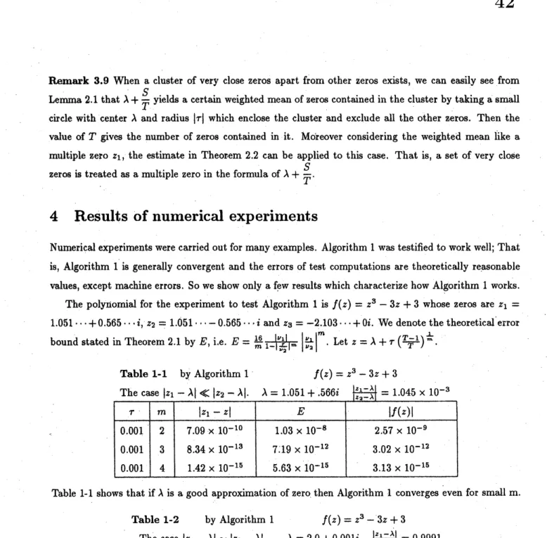
forfixed $m$and $\tau$Remark 3.9 When a cluster ofvery close zeros apart fromother zeros exists, we can easily see from Lemma
2.1
that $\lambda+\frac{S}{T}$yieldsacertainweightedmeanofzeroscontainedin thecluster bytakinga$8\mathrm{m}\mathrm{a}\mathrm{U}$circle with center $\lambda$ and radius $|\tau|$ which enclose the cluster and exclude all the other zeros. Then the
value of$T$ gives the number ofzeros contained in it. Moreover considering the weighted mean like a
multiple
zero
$z_{1}$, theestimate
in Theor$e\mathrm{m}2.2$ can be applied to this case. That is, a set ofvery closezeros istreatedas amultiple zero in the formulaof$\lambda+\frac{S}{T}$.
4
Results
of
numerical experiments
Numericalexperimentswerecarriedoutfor manyexamples. Algorithm 1 was testified to work$\mathrm{w}\mathrm{e}\mathrm{l}\mathrm{l}|$ That
is, Algorithm 1 is generally convergent and the errors of test computations are theoreticallyreasonable
values, exceptmachine $\mathrm{e}\mathrm{r}\mathrm{r}\mathrm{o}\mathrm{r}8$. Sowe show onlya$\mathrm{f},\mathrm{e}\mathrm{w}$results which characterize how Algorithm 1 works.
The polynomial for the experiment to test Algorithm 1 is $f(z)=z^{3}-3z+3$ whose zeros are $z_{1}=$
$1.051\cdots+0.565\cdots i,$ $z_{2}=1.0’ 51\cdots-0.565\cdots i$ and$z_{3}=-2.103\cdots+0i$
.
Wedenotethetheoreticalerrorboundstated in Theorem 2.1 by $E$, i.e. $E= \frac{16}{m}\frac{|\nu_{1}|}{1-1_{\dot{\nu}_{2}}^{L}|^{n}}$
.
Let $z= \lambda+\tau(\frac{T-1}{T})^{\perp}m$.
Tahlr 1-1 hv Alnnrit.hm 1 $f[_{Z})=\mathrm{z}^{3}-.\mathrm{q}_{z}\neq.\mathrm{q}$
Table 1-1 showsthat if$\lambda$ is agood approximationofzero then Algorithm 1 converges $e$venfor small $\mathrm{m}$
.
$r\mathrm{p}_{B*}\mathrm{h}\iota‘*1_{-}?arrow$ hv $\mathrm{A}1\sigma\cap 1\mathrm{i}\mathrm{t}.\mathrm{h}\mathfrak{m}1$ $f[,)=r^{3}.-.\mathrm{q}_{r}$
.$\lrcorner_{-}.\mathrm{q}$
We can seee in Table 1-2 that if $\frac{|z_{1}-\lambda 1}{\mathrm{I}^{z_{2^{-}}\lambda}1}\sim 1$ then, though $\mathrm{i}\mathrm{t}$needs a large amount ofcomputation, it
converges$\mathrm{v}e$ry slowly.
As for the examples for Algorithm 2, we tried some polynomials of order higher than 100 with
satisfactory results, added to many ones oflower order. Here we show some results which illustrate how the convergent process of Algorithm 2 is. In these experiments roughly determined $\tau$ such that
$\}\tau|=O(|f(\lambda)|)$ isused. Table 2-1 shows that Algorithm 2converges even if $|\nu_{1}|=|\nu_{2}|$
.
Table 2-2 is theresult for$f(z)=z^{20}+1$ which has simplezerosdistributed on the unit circle. Table 2-3 is theresult for
a polynomial which has doublezeros. Weset the range of$n_{1}\{1,2,3\}$ in these experiments. It is easily
seenfromourtheorems that if$|z_{1}-\dot{\lambda}|<|\tau|$ then
$\lambda+\frac{s}{T}$ approximates $z_{1}$ better than $\lambda+r(\frac{T-n}{T}\mathrm{L})^{\frac{1}{m}}$
.
Sowe added to the result of Algorithm 2 thevalue $|f( \lambda+\frac{s}{T})|$ in thefollowing tables to compare two values.
$\lambda_{6}$ inTable 2-2 iseqaul tothe exact zero to thefull digits. Notethat $\lambda_{2}+\#$in Table 2-1 and
$\lambda_{4}+\dot{F}$’ in $\mathrm{T}\mathrm{a}\mathrm{b}1\tilde{e}2,2$ can be consideredto bethe numerical solutions.
Remark 4.1Since $\lambda_{k-1}+\frac{s}{T}$can becomputed cheaply byadding oneprocess toAlgorithm2,we can
Table
2-3
$‘ \mathrm{s}\mathrm{h}_{0}\mathrm{w}8$thatinthecaseofzeros of multiplicitygreaterthan 1,our methodhasthe advantage of
rapidity and ofaccuracyover Newton’s method.
5
Concluding remarks
&mark
5.1 The feature ofour algorithm 1 and 2$\mathrm{i}_{8}$ intheusageof the error ofthenumerical integralof (1.1). Our root finding method is a new one which we cannnot find in preceding papers cited in
$\mathrm{M}\mathrm{c}\mathrm{N}\mathrm{a}\mathrm{m}\mathrm{e}\mathrm{e}’ \mathrm{S}$ biblography.
Remark 5.2 Our fundamental algorithm is provedto be globally convergentfor almostall initialvalues,
whileour applied algorithm isnot proved,yet. But we have the conjecture that Algorithm2 isglobally
convergent from thetheoreticalsituation and theresults of the numerical $\mathrm{e}\mathrm{x}\mathrm{p}\mathrm{e}\mathrm{r}\mathrm{i}\mathrm{m}\mathrm{e}\mathrm{n}\mathrm{t}8$
.
Remark 5.3 Comparing with the Newton’s metho$\mathrm{d}$
,’ Algorithm2 is comparable in rapidity andisequal
or better in accuracy, especiallyforzerosofmultiplicity greaterthan 1.
Remark 5.4 Connecting Algorithm2 and the value $\lambda+\frac{S}{T}$, the morerapid and reliable algorithm will
berealized. Comparingthe two kinds ofestimates in twc theorems, we canexpect tofind themethodto
distinguish the multiple zerosfrom the close ones.
References
[1] Atkinson, Kendall E. An introduction to NUMERICAL ANALYSIS, 2nd ed., John Wiley
&Sons,
NewYork (1987).
[2] Delves, L. M. &Lyness,J.N., ANumericalMethodforLocating the Zeros of anAnalytic Function,
Math. Comput., 21 (1967) 543-560.
[3] Henrici, P., Appliedandcomputational complex analysisVoll,Wiley$\mathrm{I}\mathrm{n}\mathrm{t}\mathrm{e}\mathrm{r}\mathrm{S}\mathrm{C}\mathrm{i}\mathrm{e}^{r}\mathrm{n}$
ce, New York (1974). [4] McMullen, C.,Familiesofrational mapsanditerative root-findingalgorithms,Ann.Math. 125(1987)
467-793.
[5] Noda,M.