JAIST Repository: Polarity Classification of Imbalanced Microblog Texts

全文

(1)JAIST Repository https://dspace.jaist.ac.jp/. Title. Polarity Classification of Imbalanced Microblog Texts. Author(s). XIANG, YUNMIN. Citation Issue Date. 2019-06. Type. Thesis or Dissertation. Text version. author. URL. http://hdl.handle.net/10119/16047. Rights Description. Supervisor:Shirai Kiyoaki, 先端科学技術研究科, 修士（情報科学）. Japan Advanced Institute of Science and Technology.

(2) Master’s Thesis. Polarity Classification of Imbalanced Microblog Texts. 1710250. XIANG YUNMIN. Supervisor Kiyoaki Shirai Main Examiner Kiyoaki Shirai Examiners Satoshi Tojo Minh Le Nguyen Shogo Okada. Graduate School of Advanced Science and Technology Japan Advanced Institute of Science and Technology (Information Science). May 2019.

(3) Abstract Sentiment analysis is a process to analyze opinion or emotion in texts. Polarity classification is one of the major problems in sentiment analysis. It is a task to classify a given text into negative, positive, or neutral. Many researchers have devoted to studies of the polarity classification. Especially, the polarity classification of texts on microblog such as Twitter is paid much attention, since users actively express their opinion on social media. However, most datasets used in past studies are balanced, in which the number of samples of each class is almost the same. However, the distribution of the polarity of texts is actually imbalanced in real social media, that is the number of neutral samples are much more than other classes. Supervised machine learning usually performs poorly on imbalanced data, since a classifier tends to judge minority samples as majority class. However, detection of minority samples (i.e. positive and negative) is important because they provide useful information for users. Over-sampling is a technique to train an accurate classifier from an imbalanced data. It increases an amount of minority samples so that the distribution of the classes is well balanced. Among various over-sampling methods, SMOTE and ADASYN are widely used. Supposing that each sample in a dataset is represented as a feature vector, SMOTE synthesizes new minority samples by randomly choosing a vector that is on a line between two existing minority samples in vector space. ADASYN is an extended version of SMOTE. It focuses on the fact that the samples nearby the other classes are difficult to be classified. Therefore, ADASYN generates more synthetic samples from minority samples near the borderline. The goal of this research is to train an accurate model that can classify polarity of a given text in an imbalanced data set. We focus on the polarity classification of texts in Twitter. We conducted a preliminary survey to reveal the distribution of the polarity in Twitter, and confirmed that 86% of tweets were neutral. It means that training a classier from an imbalance data is an important problem for the polarity classification of tweets. This thesis proposes several methods to extend SMOTE and ADASYN to improve the performance of the polarity classification in microblog. First, a novel over-sampling method called Amount Control Over-sampling (ACO) is proposed. One of the problems of SMOTE and ADASYN is that the synthetic samples are artificially generated and not real samples at all. The excessive number of synthetic samples may lead the poor performance of the polarity classification. Therefore, we propose ACO to control or optimize.

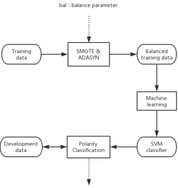
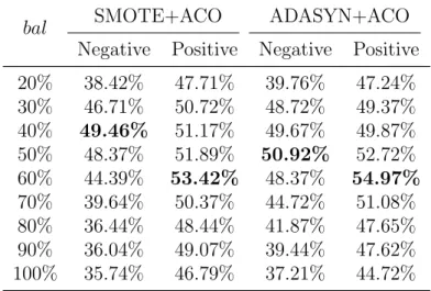
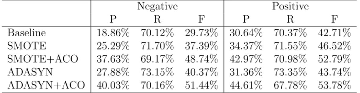
(4) the number of synthetic samples. The basic idea of ACO is to optimize the balance parameter bal on the development data. It is defined as the proportion of the minority samples to the majority samples in a new (over-sampled) data set. The balance parameter is optimized on a development data. First, for a given bal, the training data is balanced by SMOTE or ADASYN. Next, a classifier is trained on the balanced training data and applied to determine polarity labels of samples in the development data. The above procedure is repeated by changing the value of bal. The optimized bal is chosen so that F1-measure on the development data become the highest. A polarity word is a word that expresses positive or negative opinions such as “good” and “bad”. Many studies proved that polarity words were effective features for the polarity classification. Therefore, we propose an oversampling method that considers the importance of polarity words. The core idea of this method is to generate more samples from those samples that include polarity words. A weight parameter named wp is defined as the weight of samples including polarity words. More precisely, wp is a ratio of the number of synthesized samples generated from a minority sample with polarity words to that from a sample without polarity words. It is optimized on the development data. This method is called Polarity Oriented Over-sampling (POO). In addition, since the computational costs of determining wp by using trial and error on a development data is high, we propose a method to automatically determine the parameter wp. We measure the intensity of the sentiment expressed in a tweet by calculating average of sentiment scores of the words. We use a sentiment lexicon to get sentiment scores of words. The higher the intensity of the sentiment of a sample is, the greater the parameter wp is set. It enable us to synthesize more samples from a minority sample that expresses strong sentiment. This method is called as Polarity Intensity Oriented Over-sampling (PIOO). Support Vector Machine (SVM) is used to train a polarity classifier in this study. Word embedding is used to obtain a feature vector of a tweet. A weighted sum of word vectors is defined as a feature vector of a tweet. Skip-gram is applied to train word embedding. Several experiments are conducted to evaluate our methods. An imbalanced data set is constructed by adding neutral tweets to SemEval 2017 data set. First, our proposed ACO is evaluated. F1-measure of SMOTE+ACO is 48.74% and 52.79% for the negative and positive classification, which are 11.35 and 6.27 points better than SMOTE, respectively. F1-measure of ADASYN+ACO is 51.44% and 53.78% for the negative and positive classification, which are 11.07 and 10.04 points better than ADASYN, respectively. These results indicate that ACO, the method to optimize the number of synthesized samples, is effective. Next, our proposed POO is evaluated. F1-.

(5) measure of SMOTE+POO is 54.07% and 57.94% for the negative and positive classification, which are 5.33 and 5.15 points better than SMOTE+ACO, respectively. F1-measure of ADASYN+POO is 54.93% and 65.03% for the negative and positive classification, which are 3.49 and 11.25 points better than ADASYN+ACO, respectively. Therefore, POO can contribute to boost the performance of the polarity classification. Finally, our proposed PIOO is evaluated. F1-measure of ADASYN+PIOO is 52.84% and 63.49% for the negative and positive classification, which are 2.09 and 1.34 points worse than ADASYN+POO, respectively. According to the results of our experiments, PIOO could not contribute to improve the performance. We will explore anther solution to automatically determine wp with less computational costs than POO in future. We also notice that several errors are caused by ignoring the semantic features of sentence. Not only words or word embedding but also semantic relations in a tweet should be used as features for the polarity classification..

(6) Acknowledgement I would like to express my deepest gratitude to my supervisor, Associate Professor Kiyoaki Shirai, for his constant encouragement and patient guidance for my research. His scholarly attainments and diligence always inspired me. Without his support, I could not finish my research on time. It was my honored to work with him. I also would like to thank Professor Satoshi Tojo and Associate Professor Minh Le Nguyen for their valuable advice and comments towards my research. I also want to express my grateful thanks to all members of Lab Shirai and Lab Hasegawa. They not only encouraged me when I was stuck but also gave me inspiration for my study. I also learned a lot about communication skills from them. A special thank is to Zhang Yuzhi, my girlfriend. She always believes in me and supports me. Her gentlest care is one of my motivations to finish my research. She also helps me in my English. It is my pleasure to meet her. Finally, I want to give a hug to my family, my mom and my dad. Their unconditional love and constant supports gave me courage to come to JAIST for my master degree, so that I could chase my dream in my life. Without them, I could not beat the pressure I faced.. 1.

(7) Contents 1 Introduction 1.1 Background . . . . . . . . . . . . . . . . . . . . . . . . . . . . 1.2 Goals . . . . . . . . . . . . . . . . . . . . . . . . . . . . . . . . 1.3 Outline of thesis . . . . . . . . . . . . . . . . . . . . . . . . . .. 1 1 2 3. 2 Related Work 2.1 Sentiment analysis . . . . . . . . . . . . . . . . . . . . . . . . 2.1.1 Lexicon based methods for sentiment analysis . . . . . 2.1.2 Machine learning based methods for sentiment analysis 2.2 Over-sampling . . . . . . . . . . . . . . . . . . . . . . . . . . . 2.2.1 SMOTE (Synthetic Minority Oversampling TEchnique) 2.2.2 ADASYN(ADAptive SYNthetic Sampling) . . . . . . . 2.3 Word embedding . . . . . . . . . . . . . . . . . . . . . . . . . 2.4 Characteristic of this study . . . . . . . . . . . . . . . . . . . .. 4 4 5 8 10 11 12 15 16. 3 Preliminary Survey 17 3.1 Goals of this survey . . . . . . . . . . . . . . . . . . . . . . . . 17 3.2 Procedure . . . . . . . . . . . . . . . . . . . . . . . . . . . . . 18 3.3 Result and discussion . . . . . . . . . . . . . . . . . . . . . . . 19 4 Proposed Method 4.1 Polarity Classifier . . . . . . . . . . . . . . . . . . . . . . . . . 4.2 Modification of SMOTE and ADASYN . . . . . . . . . . . . . 4.3 Optimization of the number of synthetic samples . . . . . . . 4.3.1 Motivation . . . . . . . . . . . . . . . . . . . . . . . . . 4.3.2 Amount Control Oversampling (ACO) . . . . . . . . . 4.4 Oversampling methods considering polarity words . . . . . . . 4.4.1 SMOTE with Polarity Oriented Over-sampling (POO) 4.4.2 ADASYN with Polarity Oriented Oversampling (POO) 4.4.3 ADASYN with Polarity Intensity Oriented Oversampling (PIOO) . . . . . . . . . . . . . . . . . . . . . . . i. 20 20 21 24 24 27 28 29 29 31.

(8) 5 Evaluation 5.1 Data . . . . . . . . . . . . . . 5.2 Evaluation metrics . . . . . . 5.3 Evaluation of ACO . . . . . . 5.3.1 Experiment setting . . 5.3.2 Result and discussion . 5.4 Evaluation of POO and PIOO 5.4.1 Experimental setting . 5.4.2 Result and discussion . 5.5 Error analysis . . . . . . . . .. . . . . . . . . .. . . . . . . . . .. . . . . . . . . .. . . . . . . . . .. . . . . . . . . .. . . . . . . . . .. . . . . . . . . .. . . . . . . . . .. . . . . . . . . .. . . . . . . . . .. . . . . . . . . .. . . . . . . . . .. . . . . . . . . .. . . . . . . . . .. . . . . . . . . .. . . . . . . . . .. . . . . . . . . .. . . . . . . . . .. 36 36 37 39 39 39 42 42 43 44. 6 Conclusion 47 6.1 Summary . . . . . . . . . . . . . . . . . . . . . . . . . . . . . 47 6.2 Future work . . . . . . . . . . . . . . . . . . . . . . . . . . . . 48. ii.

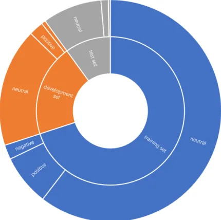
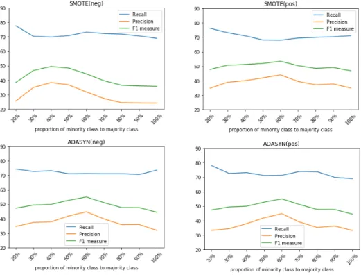
(9) List of Figures 2.1 2.2. Procedures to generate samples by SMOTE . . . . . . . . . . 11 Example of over-sampling by ADASYN . . . . . . . . . . . . . 15. 4.1 4.2 4.3. Scatter plot of original data . . . . . . . . . . . . . . . . . . . 26 Scatter plot of over-sampled data . . . . . . . . . . . . . . . . 26 Flowchart of measuring F1 score on development data in ACO 28. 5.1 5.2. Statistics of training, development and test data in chart . . . 38 Results of ACO methods on development data . . . . . . . . . 41. iii.

(10) List of Tables 3.1 3.2. Distribution of classes for each topic . . . . . . . . . . . . . . 19 Proportion of tweets with polarity words . . . . . . . . . . . . 19. 5.1 5.2 5.3. The distribution of imbalanced data set . . . . . . . . . . . . Statistics of training, development and test data . . . . . . . F1-measure of SMOTE+ACO and ADASYN+ACO on development data . . . . . . . . . . . . . . . . . . . . . . . . . . . Summary of optimized balance parameter bal . . . . . . . . Results of methods with ACO on test data . . . . . . . . . . F1-measure of SMOTE+POO and ADASYN+POO on development data . . . . . . . . . . . . . . . . . . . . . . . . . . . Comparison of POO and PIOO on development data . . . . Results of methods with POO and PIOO on test data . . . . Example of errors . . . . . . . . . . . . . . . . . . . . . . . .. 5.4 5.5 5.6 5.7 5.8 5.9. iv. . 37 . 37 . 40 . 40 . 42 . . . .. 43 44 44 46.

(11) Chapter 1 Introduction In this chapter, we first explain a background of our research in Section 1.1. Motivation and goal of this work is described in Section 1.2. Finally, the structure of the thesis is given in Section 1.3.. 1.1. Background. Sentiment analysis is the process of deriving the attitudes and opinions expressed in text data. It can be used to categorize subjective statements as positive, negative, or neutral in order to determine opinions or sentiment about a topic. It is very useful to help a user to make decision. Potential customers can know advantages and drawbacks of a product or service before purchasing or using it by reading reviews from other users. On the other hand, enterprises can know opinions from users to help them improve the quality of their products or services. With the quick development of social media, people can easily express their feeling or opinions about a product or service. More than 72% of Internet users are active on social media every day, and in such a social network, anyone generates a lot of data at any places and time. The cross-language, cross-domain, and cross-border nature of social media communication attracts a large number of users to discuss, analyze, and think about thematic events, and each user expresses his/her opinions and emotion. This leads to difficulty in monitoring and analyzing information of users’ opinions manually because there is a huge amount of opinionated text on the social media. Therefore, automated opinion mining and summarization systems are needed. Instead of using manual methods, researchers become more interested in analyzing opinionated text automatically. One of the typical problems of sentiment analysis on social media is polar1.

(12) ity classification. It is a task to classify a given text or sentence into positive, negative or neutral. More precisely, an opinion toward a target product or service expressed in a text is classified into three classes. A typical solution of classification is using machine learning. Many machine learning models are used in this task, such as Support Vector Machine(SVM), Naive Bayes, random forest, and deep neural networks. These methods made great progress in improving the performance. Most of past studies of machine learning based polarity classification assume that the data set are balanced, that is, the number of samples of each class (positive, negative or neutral) is almost the same. However, in the real-world applications, as several researches indicated, the tweets are usually present a skewed polarity distribution [1] [23]. Namely, the number of neutral samples are much more than the others. This will lead the poor performance for a machine learning based method. Let us suppose that 90% of data samples are neutral, while 10% are positive or negative. A machine learning based method tends to predict an unknown sample as a majority class, i.e neutral. However, negative samples or positive samples are usually more valuable for users. That is one of the reasons why machine learning based methods are not effective in real-world applications. To improve the performance of machine learning in processing an imbalanced data set, over-sampling and under-sampling are commonly used [4]. The core idea of these methods is to increase the number of minority samples or decrease the numbers of majority samples so that the number of samples of each class become balanced. In these approaches, how to minimize the loss of the information and how to prevent from generating too many noisy (unreliable) samples are important subjects.. 1.2. Goals. The goal of this research is to propose a method to train an accurate model that can classify polarity of a given text from an imbalanced data set. We applied a synthetic over-sampling strategy for sentiment analysis. As mentioned before, an important subject of over-sampling is that how to avoid generating too many noisy samples. In an over-sampling method, new data samples of a minority class are automatically synthesized and added to a data set. However, more data is synthesized, more noisy samples are likely to be added. There is no doubt that such noisy samples will cause the poor performance of a machine learning method. Therefore, the first goal of this research is to find a feasible way to control the number of synthetic samples. Moreover, many previous studies proved that sentiment words took an important role in sentiment analysis. A sentiment word, which is also called 2.

(13) polarity word, is a word that expresses a sentiment, emotion or polarity of an author, such as “good”, “excellent”, “bad” and “NG”. A sentiment lexicon, which is a list of sentiment words with their polarity and polarity scores, is widely used in both lexicon based methods and machine learning based methods. Drawing on the idea of considering polarity words in the sentiment analysis, we will find a feasible solution to incorporate the information of sentiment words into an over-sampling strategy. Finally, we will combine the proposed two ideas to one model to for further improvement. We will also empirically evaluate our proposed models to prove significance and credibility of them.. 1.3. Outline of thesis. The rest of the thesis is organized as follows. Chapter 2 discusses related work about sentiment analysis and over-sampling strategy. Chapter 3 presents a preliminary survey about a distribution of polarity classes on real social media. Chapter 4 explains details of our proposed methods. We presents how to improve existing over-sampling methods by quantity control of synthetic samples and considering the effectiveness of polarity words. Chapter 5 reports an evaluation of our proposed methods. Finally, Chapter 6 concludes this thesis.. 3.

(14) Chapter 2 Related Work This chapter consists of 4 sections. In Section 2.1, we take a brief look at definition of sentiment analysis, then introduce two major approaches for it. In Section 2.2, we introduce over-sampling, a commonly used technique for processing imbalanced datasets, and describe two well-known algorithms: SMOTE (Synthetic Minority Oversampling TEchnique) and ADASYN (ADAptive SYNthetic sampling). In Section 2.3 we describe the word embedding method used for this study. Finally, in Section 2.4, we clarify characteristic of this study.. 2.1. Sentiment analysis. Sentiment analysis is broadly defined as the computational study of opinions, sentiments and emotions expressed in texts. Liu et al. claimed that opinions can be classified into the following two types [15]. • Direct opinion It is an opinion explictly expressed in a text. It can be represented as a quintuple (ei ; aij ; ooijkl ; hk ; tl ) where ei is the name of an entity, aij is an aspect of ei , ooijkl is the orientation of the opinion about aspect aij of entity ei , hk is the opinion holder, and tl is the time when the opinion is expressed by hk . The opinion orientation ooijkl can be “positive”, “negative” or “neutral”, or be expressed with different strength/intensity levels. • Comparative opinion It expresses a relation of similarities or differences between two or more objects, and/or preferences in objects of the opinion holder based on some of the shared features of the objects. 4.

(15) In the past studies of sentiment analysis, direct opinions are more considered than comparative opinions. A goal of sentiment analysis or opinion mining for direct opinions can be defined as follows. Given an opinionated document d, discover all opinion quintuples (ei ; aij ; ooijkl ; hk ; tl ) in d, and identify all the synonyms and feature indicators of each feature in d. (quoted from the paper [15]) It should be stressed that the five pieces of information in the quintuple need to correspond to one another. That is, the opinion ooijkl must be given by opinion holder hk of object oj at time tl . There are commonly two kind of methods: lexicon based methods and machine learning based methods.. 2.1.1. Lexicon based methods for sentiment analysis. A lexicon based method is a traditional approach to sentiment analysis. It is based on a sentiment lexicon consisting of positive and negative words. In a sentiment lexicon, each word that represents emotion usually has a corresponding positive or negative sentiment value [22]. Researchers have proposed various ways to create such lexicons, such as automatic approach and manual approach. Using a sentiment lexicon, polarity of a given sentence or text is determined by the so-called bag-of-words model [21]. A text is viewed as a bag containing a bunch of words and phrases, regardless of the word order and grammar of the original text while keeping the frequency of the usage of each word and phrase. By looking up a sentiment lexicon, only sentiment words are picked up from a bag-of-words. For each sentiment word, positive score or negative score is also retrieved from a lexicon. The overall positive score and negative score are measured from sentiment scores of individual words by calculating sum or average. The final result of the calculation is used to determine an overall polarity for the given text. Denecke employed SentiWordNet for the multilingual sentiment analysis task [6]. SentiWordNet is a sentiment lexicon consisting of English words with three kinds of poralirty oriented scores: positive, negative and neutral scores. The first step was translation. A target document which was written in a language other than English was translated into English using standard translating softwares. Then, sentiment-bearing words, such as adjectives, were being searched and picked out. These words then went through a orientation-judging process in which each of them were paired up with a certain score indicating whether they were positive, negative, or neutral, according to SentiWordNet. Finally, the polarity of the document was determined based on the scores of sentiment words. This method was tested for German movie reviews in Amazon, and then compared to a statistical 5.

(16) polarity classifier based on n-grams. The accuracy of the proposed method reached 54%, which means that the sentiment scores from SentiWordNet were effective for this task. Taboada et al. proposed the Semantic Orientation CALculator (SOCAL), and applied it to polarity classification task [19]. It used dictionaries of words annotated with their semantic orientation, i.e. polarity and strength. SO-CAL analyzed the polarity strength scores of words and determined the polarity of a text while taking negation and intensification into consideration. This method achieved a high 78.84% accuracy for polarity classification tasks. There were also several attempts to combine lexicon-based and machine learning-based methods. Zhang et al. proposed an augmented dictionarybased method for sentiment analysis of microblogs, especially Twitter [26]. They introduced sentence type detection as a special step for analysing tweets. They defined three main sentence types to be detected in tweets: 1) Declarative Sentence: This sentence type is a direct statement of attitude or opinion that an author expresses. 2) Imperative Sentence: This sentence type involves a certain command or request. 3) Interrogative Sentence: This sentence type is a question. Since the third type of sentences did not express any opinions and usually caused classification errors, they employed a pattern matching rules to detect and remove them from datasets as follows: “model word + auxiliary verb + . . .” “. . .+ question mark” (quoted from the paper [26] ) where “model word” is a wh-word that belongs to the word set {what, where, when, who, how} and an auxiliary verb belongs to the word set {am, is, are, was, were, do, did, does}. The initial sentiment lexicon they used was one developed by Ding et al. [7]. Then, the lexicon was expanded and enriched with numerous Twitter hashtags that showed an emotional tendency or expressed opinions, such as “#bestdayever”, “#tasty”, and “#lifesucks”. With the extended sentiment lexicon, the polarity score of an entity e was calculated as X wi · so (2.1) score(e) = T wi :wi ∈L wi ∈s dis(wi , e) 6.

(17) , where wi was an opinion word, L was the sentiment lexicon, s is the sentence that contained the entity e, and dis(wi , e) was the distance between entity e and polarity word wi in the sentence s. wi · so was the semantic orientation score of wi in L. Equation (2.1) was able to calculate a semantic orientation score for the entity e so that opinion words that were closer to the entity in the sentence was weighted more than ones far away from the entity. In addition, the following heuristic rules were applied for accurate polarity classification. • Negation rules Generally speaking, in most cases a negation word or phrase, such as “no” and “not”, flips the meaning over in a sentence. Their appearance reverses the opinion or emotional tendency shown by the succeeding opinion words. Let us consider the example sentence “this cell phone is not good.” Although “good” is a positive word and is located near the entity “cell phone”, the negation word “not” turns the polarity of this sentence from positive to negative. • But-clause rules Sentences containing adversative conjunctions also require special attention when being processed and evaluated. Common adversative conjunctions are “but”, “except that”, “although”, “nevertheless”, and so on. Opinions expressed before an adversative conjunction is often opposite to what is expressed after the adversative conjunction, but either opinion is more emphasized. If “but” or “nevertheless” is appeared in the sentence, the opinion expressed after the adversative conjunction is prior to one before the conjunction. On the other hand, if “although” or “though” is used, the opinion expressed before the adversative conjunction is more emphasized. In this way, this rule depends on an adversative conjunction used in the tweets. • Decreasing and increasing rules This set of rules are applied when there exists a word that means a change of quantity or level in a sentence. Such words often imply increasing or decreasing, which can have a significant effect on the semantic orientation of the sentence. Let us consider an example sentence “The medicine I took greatly eased my pain.” Although “pain” is a negative word, the verb “eased” shows a change of level, a decrease in pain, which indicates that the writer of this sentence is satisfied with the effect of the medicine being mentioned. Because of lexicon-based approach in sentiment analysis tends to give high precision but low recall, they used texts classified by the above lexicon-based 7.

(18) method as a training set and trained a classifier by supervised machine learning with it. The obtained classifier was used to assign polarity to the entities in new tweets. The prediction accuracy of their method was 85.4%.. 2.1.2. Machine learning based methods for sentiment analysis. Supervised machine learning is widely applied for sentiment analysis. This subsection introduces several past studies. Pang and Lee used Naive Bayes, SVM, and Maximum Entropy to classify the sentiment polarity of a given movie review [18]. In the Naive Bayes, given a document d, the polarity class of d is determined as c∗ = arg max P (c|d). P (c|d) is calcurated by Bayes’ rule: P (c)P (d|c) (2.2) P (c|d) = P (d) In this formula, P (d) does not have any effect upon the selection of c∗ , thus can be ignored. In order to estimate the value for P (d|c), Naive Bayes decomposes it by assumption that the features are conditionally independent of c as follows: Q ni (d) ) P (c)( m i=1 P (fi |c) (2.3) PNB = P (d) , where fi represents a feature and ni (d) represents the frequency of fi in the documents d. Maximum entropy is another machine learning algorithm widely used in natural language processing. It estimates the conditional probability PM E (c|d) from a training data. Unlike Naive Bayes, features are not supposed to be independent. That is, relations between features are considered in the probabilistic model. See the paper [2] for details. Assuming that each data is represented as a feature vector, SVM defines a hyperplane in the feature space. This hyperplane acts as a separator of data samples of two different classes, which not only separates the document vectors of two classes but also sets the margins between the two classes and the hyperplane as large as possible. In other words, the hyperplane should be set as a position that is as far away from the two classes as possible. The separate hyperplane can be determined by solving a constrained optimization problem. Let cj ∈ {−1, 1} (corresponding to positive and negative), and cj being the correct class of document dj , the solution (separate hyperplane w) ~ can be obtained as: X w ~= αj cj d~j αj ≥ 0 (2.4) j. 8.

(19) In this formula, αj is obtained by solving a dual optimization problem. d~j such that αj is greater than zero are the only document feature vectors contributing to w, ~ so they are called the support vectors. Test instances are classified by determining which side of w’s ~ hyperplane they fall on. In their experiment of the classification of positive or negative classes, SVM outperformed Naive Bayes and Maximum Entropy. The result was relatively high accuracy, i.e. 82.9%. However, this result was obtained from a balanced data set with 700 positive samples and 700 negative samples. Followed Pang and Lee’s work, Koppel and Schler tried to solve sentiment analysis by several machine learning algorithms [13]. They also focused on neutral samples which were ignored in Pang and Lee’s work. They proved that for those binary classifiers, for example SVM, if they were trained only by positive and negative samples, the neutral samples would not simply be located at somewhere in the boundary of two classes. Therefore, neutral samples were required to train a classifier that can distinguish positive, negative or neutral. Therefore, they trained the three binary classifiers as follows. 1) Using positive and negative samples to train the classifier 2) Using positive and neutral samples to train the classifier 3) Using neutral and negative samples to train the classifier To combine results of three classifiers, they made the following rules: • If a sample is classified by the first classifier and the second classifier as positive and the third classifier classified it as neutral, it is finally classified as positive. • If a sample is classified by the first classifier and the third classifier as negative and the second classifier classified it as neutral, it is finally classified as negative. • Otherwise a sample is classified as neutral. This method yielded 74.1% accuracy for one of their data sets. The accuracy was 85.5% for the other data set. Both results were better than the classifier obtained by negative and positive samples. This article clearly proved the importance of neutral samples in sentiment analysis. However, negative samples were mostly included in the data set they used, which may be inconsistent with a distribution of polarity in the real world. Gautam et al. also applied SVM and Naive Bayes with a synonym expansion technique for sentiment analysis task for Twitter [9]. Adjectives 9.

(20) were used as features for training the supervised classifiers, since they often expressed user’s positive and negative opinions. For example, “Beautiful” is extracted as unigram feature from a tweet “painting Beautiful.” Details about this step is written in the paper [20]. SVM and Naive Bayes classifiers were trained using the features extracted from the previous step. When this initial training and classification process were completed, they used WordNet to obtain synonyms of adjectives. In the database WordNet, each adjective is associated with other words. They replaced the adjectives with their synonyms. Then, they predicted polarity of the replaced sentence. Let us consider the example sentence “I am happy.” Since “happy” could be replaced with “glad” or “satisfied” by WordNet, it was classified as positive. The accuracy of their method on a balanced data set was 89.9%, which was pretty good. More recently, deep neural network was introduced to sentiment analysis. Dos Santos et al. proposed CharSCNN (Character to Sentence Convolutional Neural Network) and achieved 86.4% sentiment prediction accuracy [8]. The first layer of the network transformed words into real-valued feature vectors (embeddings) that captured morphological, syntactic and semantic information about the words. These vectors were passed to a word-level embedding matrix. After that, a convolutional based method was used to transform the word-level embedding to a character-level embedding. To extract the sentence-level representations, they used a convolutional layer to compute a feature vector for a sentence. Finally, the feature vector of the sentence was processed by two usual neural network layers, which extracted one more abstract level of representation and computed a score for each sentiment label. This work successfully gave a solution to processing rare or infrequent words in tweets. However, they did not take attention on an imbalanced dataset in a real-world application.. 2.2. Over-sampling. The difficulty of classification in an imbalanced data is caused by extremely skew distribution of classes where the number of a majority class is much greater than a minority class. In such a situation, machine learning classifiers have the tendency of classifying minority samples as majority class wrongly, which make it difficult to detect minority samples. Many results of experiments in past studies showed poor performance on imbalanced datasets. Although SVM are believed to be less affected by imbalanced datasets, several papers reported that the performance of SVM declined significantly [24] [12]. To tackle this problem, there are several solutions to learn from an imbal10.

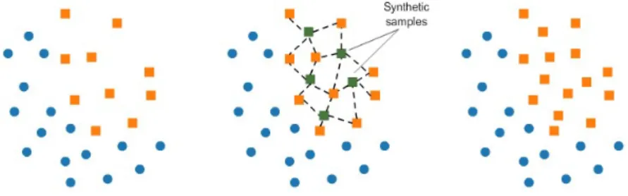
(21) anced dataset. Over-sampling is one of them. Its basic idea is to increase the numnber of samples in minority class to make the dataset become balanced. In this section, we introduce the over-sampling strategy and two famous methods: SMOTE (Synthetic Minority Oversampling TEchnique) and ADASYN (ADAptive SYNthetic sampling).. 2.2.1. SMOTE (Synthetic Minority Oversampling TEchnique). Chawla et al. proposed an over-sampling method SMOTE by synthesizing a new minority samples from existing minority samples [3]. Figure 2.1 shows how SMOTE generates synthetic samples. The squares in this figure represent the minority samples and circles represent the majority samples. The left figure shows an original distribution of data samples. The medium figure shows steps of SMOTE. First, one minority sample is randomly chosen. Second, its k nearest neighbors of minority samples are retrieved, then one of them is randomly chosen. Third, a line between a minority sample and its chosen neighbors is drawn, then a point at somewhere on the line is chosen. The vector at the point is generated as new minority samples. In other words, new minority sample is synthesized from two existing minority samples. This procedure is repeated until the number of new synthesized minority samples reaches a predefined value. The right figure in Figure 2.1 shows balanced dataset after over-sampling. Note that minority samples are generated near the region of the original minority samples. It enables a classifier to discriminate majority and minority samples easier.. Figure 2.1: Procedures to generate samples by SMOTE The pseudocode of SMOTE is shown in Algorithm 1. n is percentage of over-sampling, which is supposed to be in integral multiples of 100 (such as 100, 200 or 300). SMOTE generates the data set where the amount of minority samples are increased by n%. g is the number of samples to be synthesized from one original sample. It is determined by the formula at line 1. Smin at line 2 is a set of original minority samples. Syn is a set 11.

(22) Algorithm 1 SMOTE(X,N ,k) Input: X(original training set), n(percentage of over-sampling), k(number of nearest neighbors) Output: X 0 (new training set) 1: g ← int(n/100) 2: Smin ← a set of samples of the minority class in X 3: Syn ← φ 4: for each xi ∈ Smin do 5: Ki ← choose k nearest neighbors of xi from Smin 6: for j = 1 to g do 7: ~n ← randomly choose a sample from Ki −−→ 8: dif f ← ~n − x~i 9: gap ← random value between [0, 1] −→ − −→ ← x~ + gap × − 10: syn dif f i −→ 11: Syn ← Syn ∪ {− syn} 12: end for 13: end for 14: return X 0 = X ∪ Syn of synthetic samples to be generated; it is initialized with an empty set at line 3. For each minority sample xi in Smin , k nearest neighbors of minority samples are retrieved and collect them in a set Ki at line 5. Then, a new minority sample is synthesized as follows. A minority neighbor ~n is randomly −−→ chosen from Ki at line 7. The difference vector dif f is calculated to draw the line between x~i and ~n at line 8. A random value between [0, 1] is set as −→ −→ is determined by x~ , gap and − gap at line 9. A synthetic sample − syn dif f i −→ stands for a point somewhere on the line between x~ and ~n. at line 10. − syn i −→ is added to the set Syn at line 11. The procedures from line 7 to Then, − syn 11 are repeated g times, so that the number of synthesized minority samples becomes g × |Smin |. Finally, a union of original samples and synthetic sample is returned as a new training set X 0 at line 14.. 2.2.2. ADASYN(ADAptive SYNthetic Sampling). Based on the idea of SMOTE, various over-sampling methods have been introduced later on such as SMOTEBoost, Borderline-SMOTE and ADASYN, which all have been shown improvement on machine learning on imbalanced datasets. Han et al. claimed that a classifier was more likely to wrongly classify samples close to the borderline of different classes [10]. Thus sam12.

(23) ples near the borderline are more important for training a classifier. Based on this idea, Borderline-SMOTE was proposed. They classified data samples into the following three types: 1) all of the k nearest neighbors are majority samples, 2) at least half of the k nearest neighbors are minority samples, 3) all of the neighbors are minority samples. Borderline-SMOTE only generated samples from the second type. However, Borderline-SMOTE completely ignored the samples of which k nearest neighbors are majority samples. Inspired by Borderline-SMOTE, ADASYN was proposed by He et al. [11]. ADASYN was based on the idea of adaptively generating minority data samples according to their distributions: more synthetic data was generated for minority class samples that were harder to learn compared to those minority samples that were easier to learn. Pseudocode of ADASYN is shown in Algorithm 2. β is a desired balanced level, which is a value between 0 and 1. β = 1 means to construct a fully balanced data (the numbers of the majority and minority samples are equal), while β = 0 means no minority sample is produced. Let Smin and Smaj be a set of samples of the minority and majority classes in X at line 1 and 2, respectively. gall is the total number of samples to be synthesized. It is calculated as line 3. For each minority sample xi , its k nearest neighbors are set as nni at line 5. r[i] is the proportion of majority samples in k nearest neighbors of xi as shown at line 6. The greater r[i] is, the closer xi locates near the borderline between the majority and minority classes. rˆ[i] is normalized r[i], which can be calculated as line 9. g[i] is the number of the minority samples to be synthesized from xi , which is computed as line 10. Note that g[i] is in proportion to r[i]. It means that more minority samples are synthesized from xi near the borderline. From line 12 to 22, SMOTE is −→ except that the generation of minority applied to generate new samples − syn, samples is repeated g[i] times for xi as indicated at line 15. Finally, the union of the original training data X and synthesized data Syn is made as the new training data X 0 at line 23. The key idea of ADASYN is that the density distribution r[i] is employed to automatically determine the number of synthetic samples to be generated for each minority sample. r[i] is a measurement of the distribution of weights for different minority class samples according to their level of difficulty in learning. When there are more majority samples near a minority sample, this minority sample is supposed to be harder to be distinguished with the majority class. Such a minority sample is more weighted in the density distribution r[i] so that more new minority samples are synthesized. The resulting data set after being processed by ADASYN will show a balanced representation of the data distribution. Furthermore, it will also force the learning algorithm to focus on classification of those difficult samples near the 13.

(24) Algorithm 2 ADASN(X,β,k) Input: X (original training set), β(desired balanced level), k(number of nearest neighbor) Output: X 0 (new training set) 1: Smin ← a set of samples of the minority class in X 2: Smaj ← a set of samples of the majority class in X 3: gall ← (|Smaj | − |Smin |) × β 4: for each xi ∈ Smin do 5: nni ← k nearest neighbors of xi in X |nni ∩ Smaj | 6: r[i] ← k 7: end for 8: for each xi ∈ Smin do r[i] 9: rˆ[i] ← P i r[i] 10: g[i] ← int(ˆ r[i] × gall ) 11: end for 12: Syn ← φ 13: for each xi ∈ Smin do 14: Ki ← choose k nearest neighbors of xi from Smin 15: for j = 1 to g[i] do 16: ~n ← randomly choose a sample from Ki −−→ 17: dif f ← ~n − x~i 18: gap ← random value between [0, 1] −→ − −→ ← x~ + gap × − 19: syn dif f i −→ 20: Syn ← Syn ∪ {− syn} 21: end for 22: end for 23: return X 0 = X ∪ Syn. 14.

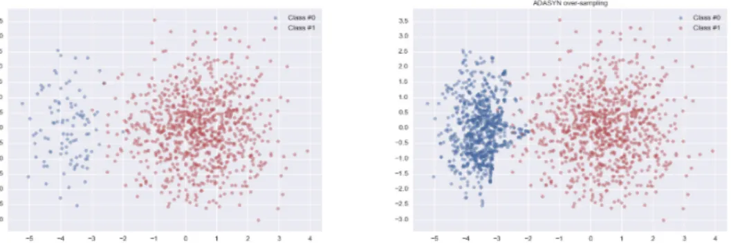
(25) borderline. This is a major difference compared to the SMOTE algorithm, in which equal numbers of synthetic samples are generated for each minority data sample. Figure 2.2 shows comparison of an original data and over-sampled data by ADASYN. The right one is the over-sampled data set and the blue points are minority samples. We can see the synthetic samples are mostly located at the borderline of two classes. This is the major difference with SMOTE, which the synthetic samples are evenly dispersed inside the minority class as shown in Figure 2.1.. Figure 2.2: Example of over-sampling by ADASYN. 2.3. Word embedding. Word embedding is known as a form of representation of words. To be more specific, they are distributed representations of words in an n-dimensional space. The usage of word embedding plays crucial and essential roles in many NLP tasks. The learned vectors explicitly encode many linguistic regularities and patterns. For example, vec(“Madrid”) - vec(“Spain”) + vec(“France”) is closer to vec(“Paris”) than to any other word vectors. Word2Vec proposed by Mikolov et al. [17] is one of the well-known tools for learning word embedding. It generates vectors by two different language models: CBOW and skip-gram. Mikolov et al. observed that the most computation part of NNLM (Neural Network Language Model) is between the non-linear layer and the softmax layer. A NNLM can be successfully trained in two steps: first is learning continuous word vectors by a simple model, and then training these distributed representations by a N-gram model, where the computational cost is large. Therefore, they removed the non-linear hidden 15.

(26) layer and let the projection layer be shared for all words. Furthermore, they also used the words from future. That is, a word was predicted by surrounding words. As the order of words in the history did not influence the projection, this model was called CBOW (Continuous Bag-of-Words Model). On the other hand, unlike CBOW, skip-gram predicted a window or context words from a single word. In this thesis, we use word embedding obtained by skip-gram as the input of the machine learning model.. 2.4. Characteristic of this study. Similar to previous studies introduced in Subsection 2.1.2, we also use machine learning method for polarity classification. Comparing with others’ work, we concentrate more on an imbalanced data set, where the number of neutral samples is much more than the number of positive or negative samples. We apply the over-sampling approach introduced in Section 2.2. Furthermore, we propose novel methods of polarity classification for an imbalanced data set by modifying existing over-sampling methods, SMOTE and ADASYN.. 16.

(27) Chapter 3 Preliminary Survey 3.1. Goals of this survey. As discussed in Chapter 1, nowadays, along with the rapid growth of the social media, many users are active on it every day. They push their feelings and experience towards someone, a product or an event. However, among these texts, only a small part of them describe opinions of users directly. Most of them just describe what the user did about a specific topic or the news about a topic. Let us consider the following two tweets. T1 Watch the new trailer for David Bowie’s ‘Blackstar’, which premieres next Thursday. T2 2nd Place again. How could it happen? #MTVSTARS Lady Gaga. T1 is a tweet about David Bowie, but it just describes that the user watched the trailer and does not express user’s opinion about David Bowie. T2 is a news about Lady Gaga. Neither opinion nor emotion is found in it. According to the definition of direct opinion we discussed in Section 2.1, T1 and T2 are treated as “neutral” samples as they do not show a direct opinion orientation towards the entity. In a review forum of an e-commercial website, there exists many opinionated sentences toward a product or service. However, in Twitter, most of tweets seem neutral as T1 and T2. Therefore, the ratio of the neutral tweets in Twitter should be empirically investigated. On the other hand, the usage of polarity words in sentiment analysis attracted many researchers’ attention. It can be a powerful feature to improve the performance of a polarity classifier. We also want to confirm whether the usage of polarity words in positive and negative tweets is significantly different with neutral samples.. 17.

(28) Considering the above, this study conducts preliminary surveys on tweets. Two objectives of the surveys are: • We will to investigate the distribution of polarity (positive, negative and neutral) of the texts in Twitter. We will confirm that the tweets in the real world are imbalanced, i.e. neutral tweets are the overwhelming majority class. This survey also helps us to construct a data set to simulate a real-world data. • We will to investigate the ratio of the tweets including polarity words in each polarity class. We will see whether the usage of polarity words is significantly different among polarity classes.. 3.2. Procedure. As for the first objective of this survey, we collect tweets by searching a keyword with Twitter API. Eight topics are chosen as a keyword, which are shown in Table 3.1. These topics are different entities, namely the movie & game (e.g. Harry Potter), electronic product (e.g. iPhone X) and celebrity (e.g. Morgan Freeman). One hundred tweets are retrieved for each topic. Thus 800 tweets are retrieved in total. Then, these tweets are manually classified in terms of their polarity toward a topic, so that we can clearly see the distribution of polarity classes. Moreover, we can also investigate whether there is significant difference on class distribution among three kinds of entities. As for the second objective of this survey, we used the data from SemEval 2017 task 4C. It is a collection of tweets about topics with polarity labels. The label indicates that the tweet expresses a positive, negative or neutral opinion toward a target topic. This data set is an extension work of SemEval 2016 task 4. It includes tweets about various topics, including people (e.g. Gadafi, Steve Jobs), products (e.g. kindle, android phone), and events (e.g. Japan earthquake, NHL playoffs). The Polarity labels are annotated by CrowdFlower or Mechanical Turk (most likely the former). We count the number of tweets with polarity words and without polarity words, so that we can see whether the ratio of the tweets with polarity words is significantly different for the polarity classes. SentiWordNet is used as a sentiment lexicon in this survey. If a sentence includes at least one polarity word in SentiWordNet, we treat it as a tweet with polarity words. If it does not include any polarity words, we consider it as a tweet without polarity words.. 18.

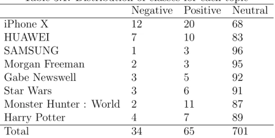
(29) 3.3. Result and discussion Table 3.1: Distribution of classes Negative iPhone X 12 HUAWEI 7 SAMSUNG 1 Morgan Freeman 2 Gabe Newswell 3 Star Wars 3 Monster Hunter : World 2 Harry Potter 4 Total 34. for each Positive 20 10 3 3 5 6 11 7 65. topic Neutral 68 83 96 95 92 91 87 89 701. Table 3.1 shows the number of negative, positive and neutral tweets about 8 topics. The last row shows the total number of tweets of all 8 topics. This table shows that the ratio of neutral tweets is quite high, 86%. On the other hands, the number of negative samples and positive samples are extremely small. Note that we did not involve the advertisement in this data set. It indicates that users usually put what they did or just state something on the social media, for example, “Bought a Harry Potter Art Piece today” and “The cast of Harry Potter is announced, 2000”. Among three kinds of entities, electronic products are mentioned with positive and negative sentences more than movie & game and celebrity. However, the proportion of neutral tweets about electronic products is still high, more than 80%. The results of Table 3.1 will be considered when we construct an imbalanced data set in the experiment. Table 3.2: Proportion of tweets with polarity words Negative Positive Number of tweets with polarity words 1933 5815 Number of tweets without polarity words 406 2397 Proportion 82.64% 70.81%. Neutral 21749 44742 32.71%. Table 3.2 shows the proportion of the tweets with polarity words for each negative, positive and neutral class. We can see there are 82.64% of negative samples include polarity words, while 70.81% of positive samples do. Only 32.71% of neutral samples include polarity words. This result indicates that the polarity words are an important component of negative and positive tweets. 19.

(30) Chapter 4 Proposed Method In this chapter, we explain details of the proposed methods for polarity classification on an imbalanced data set. Section 4.1 explains how to train the polarity classifier. Section 4.2 describes slight modification of SMOTE and ADASYN. Then, first propose a method to control or optimize the number of synthesized minority samples in over-sampling approaches. Next, we propose another over-sampling method that takes polarity words into account in synthesis of minority samples.. 4.1. Polarity Classifier. This section describes the classifier for polarity classification. Similar to the previous work, supervised machine learning is applied to train a polarity classifier. Two binary classifiers are trained: one judges whether a given tweet is positive or not (neutral), the other judges whether a tweet is negative or not (neutral). For training classifiers, tweets in a training and test data are represented as feature vectors. As for the extraction of features, word unigrams, bigrams, parts of speech and sentiment words are widely used. As for weights of features in a feature vector, information gain (IG), term frequency-inverse document frequency (TF-IDF), mutual information (MI), and the Chi-square statistic (CHI) are often used [25]. However, these statistical features are semantically weak. In addition, these features often suffer from data sparseness. If most features in a tweet in a test data do not appear in a training data, it could not be classified correctly. In this study, word embedding is used to obtain a feature vector for each tweet. Word embedding includes semantic information that cannot be captured by n-gram features. In addition, vector representation by word embedding less suffers from data sparseness. 20.

(31) A vector of a given tweet is obtained as follows. First, we perform preprocessing on a tweet. It consists of the following steps. 1. All characters in upper case are converted to lower case. 2. Stopwords are removed by NLTK1 in Python. 3. URLs are replaced with a special token “url”. 4. “@ user id” is replaced with a special token “user mention”. Next, each word in a tweet is represented by a vector using word embedding. Finally, a vector of a whole tweet is obtained by Equation (4.1). P ~i × wi iv (4.1) sentence vector = P 2 i wi v~i is the vector representation of i-th word, which is pre-trained by skip-gram model. wi is the weight for the i-th word. wi is determined by TF-IDF, as Corerea et al. mentioned [5]. We trained the vectors of words by using Tensorflow Hub2 . Tensorflow Hub is a library that provides the reusable code of machine learning methods. English Wikipedia corpus is used to train word embedding. The dimension of the word vectors is set as 250. This library assigns a zero vector for out-of-vocabulary words. Support Vector Machine (SVM) is used to train a classifier. It is a classical supervised machine learning algorithm and widely used in classification and regression. We train SVM classifier by sklearn3 , which is a powerful library for implementation of machine learning in Python. The square of the hinge loss function is chosen as the loss function for training. The penalty parameter C of the error term is set as 0.5. The kernel of SVM is linear kernel.. 4.2. Modification of SMOTE and ADASYN. Our proposed over-sampling methods are extension of SMOTE and ADASYN. The number of synthesized samples is given as input in both methods, but in different ways. In SMOTE, the percentage of over-sampling n is given in Algorithm 1. On the other hand, in ADASYN, the desired balanced level β is given in Algorithm 2. 1. http://www.nltk.org/ https://tensorflow.google.cn/hub/ 3 https://scikit-learn.org/ 2. 21.

(32) Algorithm 3 SMOTE(X,bal,k) Input: X(original training set), bal(balance parameter), k(number of nearest neighbors) Output: X 0 (new training set) 1: Smin ← a set of samples of the minority class in X 2: Smaj ← a set of samples of the majority class in X 3: gall ← |Smaj | × bal − |Smin | 4: g ← int(gall /|Smin |) 5: Syn ← φ 6: for each xi ∈ Smin do 7: Ki ← choose k nearest neighbors of xi from Smin 8: for j = 1 to g do 9: ~n ← randomly choose a sample from Ki −−→ 10: dif f ← ~n − x~i 11: gap ← random value between [0, 1] −→ − −→ ← x~ + gap × − 12: syn dif f i −→ 13: Syn ← Syn ∪ {− syn} 14: end for 15: end for 16: return X 0 = X ∪ Syn We slightly modify SMOTE and ADASYN so that we can control the number of synthesized samples in the same way. We introduce a balance parameter bal that is the proportion of the minority samples to the majority samples in a new (over-sampled) data set. For example, bal = 1 means that the new training data contains the equal number of majority and minority samples, while bal = 0.5 means that the amount of the minority samples becomes 50% of the majority samples. Pseudocode of our modified SMOTE and ADASYN are shown in Algorithm 3 and Algorithm 4, respectively. In the modified SMOTE, g (the number of minority samples to be synthesized from one original sample) is calculated as line 4 in Algorithm 3 instead of line 1 in Algorithm 1. gall means the total number of minority samples to be synthesized, which is calculated as line 3 so that the ratio of the number of minority samples to majority samples becomes bal. Then gall is equally divided to each minority sample as line 4. Lines from 5 to 16 are exactly same as the original SMOTE. In the modified ADASYN, gall (the total number of minority samples to be synthesized) is calculated as line 3 in Algorithm 4 instead of line 3 in. 22.

(33) Algorithm 4 ADASYN(X,bal,k) Input: X (original training set), bal(balance parameter), k(number of nearest neighbor) Output: X 0 (new training set) 1: Smin ← a set of samples of the minority class in X 2: Smaj ← a set of samples of the majority class in X 3: gall ← |Smaj | × bal − |Smin | 4: for each xi ∈ Smin do 5: nni ← k nearest neighbors of xi in X |nni ∩ Smaj | 6: r[i] ← k 7: end for 8: for each xi ∈ Smin do r[i] 9: rˆ[i] ← P i r[i] 10: g[i] ← int(ˆ r[i] × gall ) 11: end for 12: Syn ← φ 13: for each xi ∈ Smin do 14: Ki ← choose k nearest neighbors of xi from Smin 15: for j = 1 to g[i] do 16: ~n ← randomly choose a sample from Ki −−→ 17: dif f ← ~n − x~i 18: gap ← random value between [0, 1] −→ − −→ ← x~ + gap × − 19: syn dif f i −→ 20: Syn ← Syn ∪ {− syn} 21: end for 22: end for 23: return X 0 = X ∪ Syn. 23.

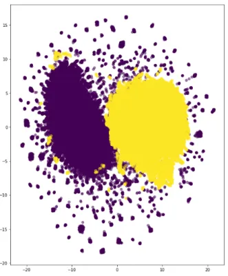
(34) Algorithm 2. Similarly, gall is determined so that the ratio of the number of minority samples to majority samples becomes bal. Lines from 4 to 23 are exactly same as the original ADASYN.. 4.3 4.3.1. Optimization of the number of synthetic samples Motivation. Our polarity classifier is based on supervised machine learning. However, imbalance of the polarity classes in a training data is an obstacle for supervised learning. A classifier trained from imbalance training data tends to misclassify a minority data as a majority data. The data imbalance problem is particularly serious in polarity classification in tweets. Our preliminary survey in Chapter 3 showed that neutral tweets appear much more than positive or negative tweets in a real world. Among existing solutions for imbalance of the data, over-sampling is the most practical and applicable to a wide range of applications. As we discussed before, however, over-sampling has weakness. That is, newly synthesized samples may be inaccurate and noisy, because they are not real samples at all. Therefore, balancing the ratio of original samples and synthesized samples is a critical subject. To see how excessive generation of minority samples influences the polarity classification, we visualize the data set before and after over-sampling. The data set consists of a few positive tweets and a lot of neutral tweets, which is constructed for our experiment4 . We use SMOTE to generate minority samples on our imbalanced data set. The bal here is set as 1, i.e. the numbers of majority and minority samples are equal after over-sampling. Then, we use tSNE (t-distributed stochastic neighbor embedding) [16], a widely used method for dimension reduction and visualization, to reduce the dimension of original training set and over-sampled training set, and then visualize them. Figure 4.1 shows the result of tSNE of original data set, while Figure 4.2 shows the result of over-sampled data set. Yellow and purple scatters represent minority and majority samples. In Figure 4.1, we can roughly see the borderline of classes, and confirm that several minority samples are mixed in majority samples. These mixed samples are commonly considered as noisy for an SVM classifier. In Figure 4.2, we can see that data set becomes balanced, but the number of noisy samples increases. This result indicates that over-sampling methods can effectively make datasets become 4. The details of this data will be explained in Section 5.1.. 24.

(35) balanced, but it also generates noisy samples. In addition, synthetic samples are not real samples at all. No one can assure such samples will not cause classification errors in machine learning. Therefore, it is necessary to control the number of synthetic samples so that datasets become relatively balanced while noisy samples are less generated.. 25.

(36) Figure 4.1: Scatter plot of original data. Figure 4.2: Scatter plot of over-sampled data 26.

(37) 4.3.2. Amount Control Oversampling (ACO). We propose a new over-sampling method called Amount Control Over-sampling (ACO). It is an extension of SMOTE and ADASYN. In SMOTE and ADASYN, the number of synthesized samples is pre-defined in ad-hoc manner. However, as discussed in Subsection 4.3.1, adding too many synthesized samples into an original data set may cause decrease of the classification performance. In ACO, the number of the synthesized samples are empirically optimized to prevent from adding too many noisy samples. Algorithm 5 ACO(Dtrain ,Ddev ,B) Input: Dtrain (training data), Ddev (development data), B = {bal1 , · · · , baln } (set of balance parameters) ˆ (optimized balance parameter) Output: bal 1: for i = 1 to |B| do b ← SMOTE(Dtrain , bali , k) 2: (1) Dtrain b 3: (2) Dtrain ← ADASYN(Dtrain , bali , k) b 4: SV M ← training SVM classifier from Dtrain 5: Ldev ← polarity labels of samples in Ddev classified by SV M 6: F1dev [i] ← F1 score of Ldev 7: end for ˆ ← bali0 where i0 = arg max F1dev [i] 8: bal ˆ 9: return bal The basic idea of ACO is to optimize the balance parameter bal on the development data. Pseudocode of ACO is shown in Algorithm 5. First, we prepare a training data Dtrain and development data Ddev . We also prepare a list of balance parameters B. Recall that the balance parameter bal determines the number of synthesized minority samples in SMOTE and ADASYN. For each balance parameter bali ∈ B, the training data is balanced by SMOTE (Algorithm 3) at line 2 or ADASYN (Algorithm 4) at line 3. Note that the parameter k is predefined. Next, SVM is trained from the balanced trainb ing data Dtrain at line 4. Then, it is applied to determine polarity labels of samples in Ddev at line 5. The F1-measure of predicted polarity labels Ldev is calculated at line 6. Finally, the optimized balance parameter is chosen so that F1dev [i] becomes the highest. Figure 4.3 illustrates how to compute F1dev [i] for a given bali .. 27.

(38) Figure 4.3: Flowchart of measuring F1 score on development data in ACO. 4.4. Oversampling methods considering polarity words. In this section, we will introduce the other proposed model that considers polarity words in over-sampling. Kousta et al. emphasized the importance of polarity words in the sentiment analysis [14]. General speaking, both negative and positive words play more important roles that neutral words in polarity classification. Inspired by previous work introduced in Section 2.1, we design a modified version of SMOTE and ADASYN that generates more synthesized samples including polarity words. In addition, according to the preliminary survey introduced in Section 3.3, there are more than 70% of minority (positive or negative) samples include polarity words, while only 30% of neutral samples do. It is a natural idea to increase the importance of. 28.

(39) those samples including polarity words in classifier learning for improvement of the performance of polarity classification. Following the above ideas, we design a modified version of SMOTE and ADASYN that generates more synthesized samples including polarity words.. 4.4.1. SMOTE with Polarity Oriented Over-sampling (POO). SMOTE is an algorithm that generates synthetic samples from minority samples. The numbers of synthesized samples are equal for all original minority samples. In our extended model, more samples are generated from those samples with polarity words. Algorithm 6 shows a pseudocode of the proposed method. A weight parameter named wp is defined as the weight of samples including polarity words. The greater the wp is, the more samples are generated from samples with polarity words. For each minority sample xi , r[i] is set as wp if xi contains polarity words, otherwise 1, as indicated in lines between 4 and 10. We use SentiWordNet to judge whether a word in a tweet is a polarity word or not. r[i] is similar to the density distribution in ADASYN; it controls the number of synthesized samples from xi . Following procedures are the same as ADASYN. r[i] is normalized as rˆ[i] at line 12, then g[i] is calcurated as line 13. The minority samples are generated g[i] times from xi in lines between 16 and 25. The parameter wp is optimized using the development data. Among a set of possible values, the best wp is chosen so that the F1-measure of the trained classifier on the development data becomes the highest. Note that wp should be a value greater than 1 to produce more samples containing polarity words. The detail procedures of the optimization is almost the same as the procedures shown in Algorithm 5 and Figure 4.3. Hereafter, Polarity Oriented Over-sampling (POO) stands for the proposed technique that generates more synthesized samples from samples including polarity words. SMOTE combined with POO (Algorithm 6) is referred as SMOTE+POO.. 4.4.2. ADASYN with Polarity Oriented Oversampling (POO). ADASYN adaptively generates samples so that more synthetic data is generated from minority samples that are harder to be discriminated from majority samples, or that locate near a border between minority and majority samples 29.

(40) Algorithm 6 SMOTE+POO(X,bal,k,wp) Input: X(original training set), bal(balance parameter), k(number of nearest neighbors), wp (weight parameter) Output: X 0 (new training set) 1: Smin ← a set of samples of the minority class in X 2: Smaj ← a set of samples of the majority class in X 3: gall ← |Smaj | × bal − |Smin | 4: for each xi ∈ Smin do 5: if xi includes a polarity word then 6: r[i] ← wp 7: else 8: r[i] ← 1 9: end if 10: end for 11: for each xi ∈ Smin do r[i] 12: rˆ[i] ← P i r[i] 13: g[i] ← int(ˆ r[i] × gall ) 14: end for 15: Syn ← φ 16: for each xi ∈ Smin do 17: Ki ← choose k nearest neighbors of xi from Smin 18: for j = 1 to g[i] do 19: ~n ← randomly choose a sample from Ki −−→ 20: dif f ← ~n − x~i 21: gap ← random value between [0, 1] −→ − −→ ← x~ + gap × − 22: syn dif f i −→ 23: Syn ← Syn ∪ {− syn} 24: end for 25: end for 26: return X 0 = X ∪ Syn. 30.

(41) in a feature space. The key step of this method is to assign each minority sample the density distribution in synthetic process as line 6 in Alrorithm 2 or Alrorithm 4. To produce more samples including polarity words, we define polarity oriented density distribution rp [i] as follows. ( wp × r[i], when xi includes polarity words rp [i] = (4.2) r[i], when xi does not include polarity words wp is a parameter that controls how many new samples are synthesized from the minority sample including polarity words. It should be a value greater than 1 to produce more samples containing polarity words. We call this method ADASYN with Polarity Oriented Over-sampling or ADASYN+POO. A pseudocode of ADASYN+POO is shown in Algorithm 7. The only difference of this algorithm and the original ADASYN is procedures from line 7 to 9. We update r[i] by multiplying wp if xi contains a polarity word. It is equivalent to Equation (4.2). Thus ADASYN+POO is able to not only generate more synthetic samples near the borderline but also create more samples from those samples with polarity words. Similar to SMOTE+POO, the parameter wp is optimized using a development data.. 4.4.3. ADASYN with Polarity Intensity Oriented Oversampling (PIOO). Another extension of ADASYN in this study is ADASYN with Polarity Intensity Oriented Over-sampling (PIOO). One of the disadvantages of POO proposed in Subsection 4.4.1 and 4.4.2 is its computational cost. Since the parameter wp is optimized on the development data, training a classifier and applying it on the development data are repeated many times. Therefore, we try to automatically determine the parameter wp without using trial and error on the development data. More concretely, we propose a method to determine wp by sentiment scores of polarity words in a tweet. First, sentiment scores of words in a tweet are calculated using SentiWordNet. In SentiWordNet, each word has positive and negative scores. These scores are values between 0 and 1. They can be zero when a word does not convey positive or negative emotion. Precisely, sentiment scores are assigned to not words but senses. Therefore, when a word has two or more senses, it has different scores in terms of its senses. The sentiment score of a word wi , SenScore(wi ), is calculated by the following steps. 1. Supposing that wi has t senses, denoted as {si1 , · · · , sit }. Averages of 31.

(42) Algorithm 7 ADASYN+POO(X,bal,k,wp) Input: X (original training set), bal(balance parameter), k(number of nearest neighbor), wp (weight parameter) Output: X 0 (new training set) 1: Smin ← a set of samples of the minority class in X 2: Smaj ← a set of samples of the majority class in X 3: gall ← |Smaj | × bal − |Smin | 4: for each xi ∈ Smin do 5: nni ← k nearest neighbors of xi in X |nni ∩ Smaj | 6: r[i] ← k 7: if xi includes a polarity word then 8: r[i] ← wp × r[i] 9: end if 10: end for 11: for each xi ∈ Smin do r[i] 12: rˆ[i] ← P i r[i] 13: g[i] ← int(ˆ r[i] × gall ) 14: end for 15: Syn ← φ 16: for each xi ∈ Smin do 17: Ki ← choose k nearest neighbors of xi from Smin 18: for j = 1 to g[i] do 19: ~n ← randomly choose a sample from Ki −−→ 20: dif f ← ~n − x~i 21: gap ← random value between [0, 1] −→ − −→ ← x~ + gap × − 22: syn dif f i −→ 23: Syn ← Syn ∪ {− syn} 24: end for 25: end for 26: return X 0 = X ∪ Syn. 32.

(43) positive and negative scores of senses are calculated as follows. Pt j=1 SW Npos (sij ) Scorepos (wi ) = (4.3) t Pt j=1 SW Nneg (sij ) (4.4) Scoreneg (wi ) = t SW Npos (sij ) and SW Nneg (sij ) are the positive and negative score of sense sij in SentiWordNet, respectively. 2. A sentiment score of a word wi is given by Equation (4.5).  if Scorepos (wi ) = Scoreneg (wi ) = 0 0 SenScore(wi ) = Scorepos (wi ) + 1 if Scorepos (wi ) ≥ Scoreneg (wi )  Scoreneg (wi ) + 1 if Scorepos (wi ) < Scoreneg (wi ) (4.5) Basically, SenScore(wi ) is defined as the higher value between averages of positive and negative scores. In addition, in order to be SenScore(wi ) greater than 1, the score is added by 1. We will explain the reason why SenScore(wi ) should be greater than 1 later. For each data sample (tweet) xi , a sentiment score s[i] is calculated as Equation (4.6). P wi ∈P W (xi ) SenScore(wi ) s[i] = (4.6) |P W (xi )| P W (xi ) stands for a set of polarity words in a tweet xi . Here a polarity word is defined as a word whose SenScore is greater than 0. That is, s[i] is an average score of sentiment scores of polarity words in a tweet. Roughly saying, s[i] evaluates intensity of sentiment of xi . Note that s[i] should be greater than one to give importance to samples with polarity words in generation of minority samples. That is the reason why we make SenScore(wi ) become greater than 1 in Equation (4.5). Then, we calculate the polarity oriented density distribution rp [i] for each minority samples as follows. ( s[i] × r[i], when xi includes polarity words rp [i] = (4.7) r[i], when xi does not include polarity words Note that wp in Equation (4.2) is replaced with s[i]. The basic idea is to synthesize more samples from a minority sample that expresses sentiment strongly. Furthermore, the number of the synthesized samples is proportion to the intensity of the sentiment of xi . Note that s[i] should be greater 33.

(44) than one to give importance to samples with polarity words in generation of minority samples. That is the reason why we make SenScore(wi ) become greater than 1 in Equation (4.5). A pseudocode of ASASYN+PIOO is shown in Algorithm 8. Only difference between ADASYN+PIOO and ADASYN+POO is procedures in lines between 7 and 10. They represent the update of r[i] that is equivalent to Equation (4.7).. 34.

(45) Algorithm 8 ADASN+PIOO(X,bal,k,wp) Input: X (original training set), bal(balance parameter), k(number of nearest neighbor), wp (weight parameter) Output: X 0 (new training set) 1: Smin ← a set of samples of the minority class in X 2: Smaj ← a set of samples of the majority class in X 3: gall ← |Smaj | × bal − |Smin | 4: for each xi ∈ Smin do 5: nni ← k nearest neighbors of xi in X |nni ∩ Smaj | 6: r[i] ← k 7: if xi includes P a polarity word then wi ∈SW (xi ) SenScore(wi ) 8: s[i] = |SW (xi )| 9: r[i] ← s[i] × r[i] 10: end if 11: end for 12: for each xi ∈ Smin do r[i] 13: rˆ[i] ← P i r[i] 14: g[i] ← int(ˆ r[i] × gall ) 15: end for 16: Syn ← φ 17: for each xi ∈ Smin do 18: Ki ← choose k nearest neighbors of xi from Smin 19: for j = 1 to g[i] do 20: ~n ← randomly choose a sample from Ki −−→ 21: dif f ← ~n − x~i 22: gap ← random value between [0, 1] −→ − −→ ← x~ + gap × − 23: syn dif f i −→ 24: Syn ← Syn ∪ {− syn} 25: end for 26: end for 27: return X 0 = X ∪ Syn. 35.

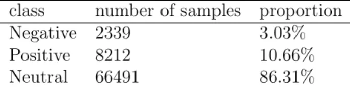
(46) Chapter 5 Evaluation This chapter reports results of experiments to evaluate our proposed methods. First, we present data sets and evaluation metric. Then, we present the performance of SMOTE and ADASYN with ACO proposed in Section 4.3, and compare them with baselines. Next, we show the performance of POO and PIOO proposed in Section 4.4, and compare them with baselines. Finally, we perform error analysis to reveal advantages and disadvantages of the proposed methods.. 5.1. Data. A benchmark data set of SemEval 2017 is used in the experiment. It is a collection of tweets about several topics with manually annotated with their polarity. Polarity of each tweet is represented as 5-scale labels from 1 (very negative) to 5 (very positive). In this experiment, we define three classes, negative, positive and neutral, as classification labels. Thus we convert 1 or 2 to “negative”, 3 to “neutral” and 4 or 5 to “positive”. The data set consists of 2,339 negative samples, 8,212 positive samples and 10,081 neutral samples. However, our preliminary survey showed that 86% tweets were neutral in Twitter. To make the distribution of the polarity labels of the data set become close to the actual distribution, we collect neutral tweets to the data set by the following procedures. 1. We retrieve tweets via Twitter API by searching the key words of topics in SemEval 2017. 2. We classify the retrieved tweet by AYLIEN1 , which is a web tool-kit for polarity classification. Only tweets classified as neutral are kept, 1. https://aylien.com/text-api/sentiment-analysis/. 36.