JAIST Repository
https://dspace.jaist.ac.jp/Title
Hardness Results and an Exact Exponential
Algorithm for the Spanning Tree Congestion
Problem
Author(s)
Okamoto, Yoshio; Otachi, Yota; Uehara, Ryuhei;
Uno, Takeaki
Citation
Lecture Notes in Computer Science, 6648/2011:
452-462
Issue Date
2011-04-27
Type
Journal Article
Text version
author
URL
http://hdl.handle.net/10119/9861
Rights
This is the author-created version of Springer,
Yoshio Okamoto, Yota Otachi, Ryuhei Uehara and
Takeaki Uno, Lecture Notes in Computer Science,
6648/2011, 2011, 452-462. The original
publication is available at www.springerlink.com,
http://dx.doi.org/10.1007/978-3-642-20877-5_44
Description
8th Annual Conference on Theory and Applications
of Medels of Computation, TAMC 2011, Tokyo,
Japan, May 23-25, 2011.
Hardness Results and an Exact Exponential Algorithm
for the Spanning Tree Congestion Problem
Yoshio Okamoto1, Yota Otachi2, Ryuhei Uehara3, and Takeaki Uno4
1 Center for Graduate Education Initiative, JAIST, Asahidai 1–1, Nomi, Ishikawa 923–1292,
Japan. [email protected]
2 Graduate School of Information Sciences, Tohoku University, Sendai 980–8579, Japan. JSPS
Research Fellow. [email protected]
3 School of Information Science, JAIST, Asahidai 1–1, Nomi, Ishikawa 923–1292, Japan.
4 National Institute of Informatics, 2–1–2 Hitotsubashi, Chiyoda-ku, Tokyo, 101–8430, Japan.
Abstract. Spanning tree congestion is a relatively new graph parameter, which
has been studied intensively. This paper studies the complexity of the problem to determine the spanning tree congestion for non-sparse graph classes, while it was investigated for some sparse graph classes before. We prove that the prob-lem is NP-hard even for chain graphs and split graphs. To cope with the hardness of the problem, we present a fast (exponential-time) exact algorithm that runs in
O∗(2n) time, where n denotes the number of vertices. Additionally, we provide a constant-factor approximation algorithm for cographs, and a linear-time algo-rithm for chordal cographs.
1
Introduction
Spanning tree congestion is a graph parameter defined by Ostrovskii [18] in 2004. Si-monson [21] also studied the same parameter under a different name as a variant of cutwidth. After Ostrovskii [18], several graph-theoretic results have been presented [2, 6, 12–17, 19], and very recently the complexity of the problem for determining the pa-rameter has been studied [3, 20]. The papa-rameter is defined as follows. Let G be a con-nected graph and T be a spanning tree of G. The detour for an edge{u, v} ∈ E(G) is a unique u–v path in T . We define the congestion of e∈ E(T), denoted by cngG,T(e), as the number of edges in G whose detours contain e. The congestion of G in T , denoted by cngG(T ), is the maximum congestion over all edges in T . The spanning tree
conges-tion of G, denoted by stc(G), is the minimum congesconges-tion over all spanning trees of G. We denote by STC the problem of determining whether a given graph has spanning tree congestion at most given k. If k is fixed, then we denote the problem by k-STC.
Bodlaender, Fomin, Golovach, Otachi, and van Leeuwen [3, 20] studied the com-plexity of STC and k-STC. They showed that k-STC is linear-time solvable for apex-minor-free graphs and bounded-degree graphs, while k-STC is NP-complete even for K6-minor-free graphs with only one vertex of unbounded degree if k ≥ 8. They also showed that STC is NP-complete for planar graphs. Bodlaender, Kozawa, Matsushima, and Otachi [2] showed that the spanning tree congestion can be determined in linear
time for outerplanar graphs. Although several complexity results are known as men-tioned above, they are restricted to sparse graphs. The complexity for non-sparse graphs such as chordal graphs and chordal bipartite graphs were unknown.
In this paper, we show that STC is NP-complete for these important non-sparse graph classes. More precisely, we show that STC is NP-complete even for chain graphs and split graphs. It is known that every chain graph is chordal bipartite, and every split graph is chordal. The hardness for chain graphs is quite unexpected, since there is no other natural graph parameter that is known to be NP-hard for chain graphs, to the best of our knowledge. The hardness for chain graphs also implies the hardness for graphs of clique-width at most three. To cope with the hardness of the problem, we present a fast exponential-time exact algorithm. Our algorithm runs in O∗(2n) time,
while a naive algorithm that examines all spanning trees runs in O∗(2m) or O∗(nn) time, where n and m denote the number of vertices and the number of edges. Note that O∗( f (n))= O( f (n) · poly(n)). The idea, which allows us to achieve this running time, is to enumerate all possible combinations of cuts instead of all spanning trees. Using this idea, we can design a dynamic-programming-based algorithm that runs in O∗(3n) time. Then, by carefully applying the fast subset convolution method developed by Björk-lund, Husfeldt, Kaski, and Koivisto [1], we finally get the running time O∗(2n). We also
study the problem on cographs. It is known that cographs are precisely the graphs of clique-width at most two. For some cographs such as complete graphs and complete p-partite graphs, the closed formulas for the spanning tree congestion are known [12, 14, 18]. Although the complexity of STC for cographs remains unsettled, we provide a constant-factor approximation algorithm for them. Furthermore, we present a linear-time algorithm for chordal cographs.
Due to space limitation all proofs are omitted.
2
Preliminaries
Graphs in this paper are finite, simple, and connected, if not explicitly stated otherwise. We deal with edge-weighted graphs in Subsections 2.2 and 3.1. Our exponential-time exact algorithm runs in O∗(2n) time for edge-weighted graphs, too.
2.1 Graphs
Let G be a connected graph. For S ⊆ V(G), we denote by G[S ] the subgraph induced by S . For an edge e∈ E(G), we denote by G − e the graph obtained from G by the deletion of e. Similarly, for a vertex v∈ V(G), we denote by G − v the graph obtained from G by the deletion of v and its incident edges. By NG(v), we denote the (open) neighborhood
of v in G; that is, NG(v) is the set of vertices adjacent to v in G. For S ⊆ V(G), we
denote∪v∈SNG(v) by NG(S ). We define the degree of v in G as degG(v)= |NG(v)|. If
degG(v)= |V(G)| − 1, then v is a universal vertex of G.
Let G and H be graphs. We say that G and H are isomorphic, and denote it by G ≃ H, if there is a bijection f : V(G) → V(H) such that {u, v} ∈ E(G) if and only if
{ f (u), f (v)} ∈ E(H). Now assume V(G) ∩ V(H) = ∅. Then the disjoint union of G and
E(G)∪ E(H). The join of G and H, denoted by G ⊕ H, is the graph with the vertex set V(G)∪ V(H) and the edge set E(G) ∪ E(H) ∪ {{u, v} | u ∈ V(G), v ∈ V(H)}.
For A, B ⊆ V(G), we define EG(A, B) = {{u, v} ∈ E(G) | u ∈ A, v ∈ B}. For S ⊆
V(G), we define the boundary edges of S , denoted byθG(S ), asθG(S )= EG(S, V(G)\S ).
Note thatθG(∅) = θG(V(G))= ∅. The congestion cngG,T(e) of an edge e∈ E(T) satisfies
cngG,T(e)= |θG(Ae)|, where Aeis the vertex set of one of the two components of T− e.
For an edge e in a tree T , we say that e separates A and B if A⊆ Aeand B⊆ Be, where
Aeand Beare the vertex sets of the two components of T− e. Clearly, if T is a spanning
tree of G and e∈ E(T) separates A and B, then cngG,T(e)≥ |E(A, B)|. If e separates A and B, we also say that e divides A∪ B into A and B.
Let T be a tree rooted at r∈ V(T). Then we denote by prtT(v) the parent of v∈ V(T)
in T . The parent of the root r is not defined. We denote by ChdT(v) the children of
v∈ V(T) in T. Clearly, NT(v)= {prtT(v)} ∪ ChdT(v) for every non-root vertex v.
2.2 Spanning tree congestion of weighted graphs
A graph G may be associated with an edge-weight function wei : E(G) → Z+. If a graph has such a function, then we call it an edge-weighted graph or just a weighted graph. Note that unweighted graphs can be considered as weighted graphs by setting wei(e) = 1 for each edge e. For an edge-weighted graph G and F ⊆ E(G), we define wei(F)=∑f∈Fwei( f ) for F⊆ E(G). We extend the notion of spanning tree congestion
to edge-weighted graphs by defining the congestion of an edge e as the sum of the weights of edges whose detours pass through the edge e. If e ∈ E(T) separates vertex sets A and B, then cngG,T(e)≥ wei(E(A, B)).
For a weighted graph G, we define the weighted degree of v in G as wdegG(v) =
wei(θG({v})). It is not difficult to see that the following fact holds.
Proposition 2.1. Let G be a weighted graph, and let S ⊆ V(G). Then
wei(θG(S ))=
∑
v∈S
wdegG(v)− 2wei(E(G[S ])).
It is known that STC for weighted graphs is equivalent to STC for unweighted graphs in the following sense.
Lemma 2.2 ([3, 20]). Let G be a weighted graph and let e∈ E(G). Let G′be the graph obtained from G by removing the edge e and adding wei(e) internally disjoint paths of arbitrary lengths between the ends of e, where each edge in the added paths is of unit weight. Then, stc(G)= stc(G′).
2.3 Graph classes
A graph is chordal if it has no induced cycle of length greater than three. A graph G is a split graph if its vertex set V(G) can be partitioned into two sets C and I so that C is a clique of G and I is an independent set of G. Clearly, every split graph is a chordal graph (see [10]). A cograph (or complement-reducible graph) is a graph that can be constructed recursively by the following rules:
1. K1is a cograph;
2. if G and H are cographs, then so is G∪ H; 3. if G and H are cographs, then so is G⊕ H.
Note that if G is a connected cograph with at least two vertices, then G can be expressed as G1⊕G2for some nonempty cographs G1and G2. A cograph is a chordal cograph if it is also a chordal graph. Chordal cographs are also known as trivially perfect graphs [4, 10] and quasi-threshold graphs [22]. It is known that in the construction of a chordal cograph by the above rules, we can assume one of two operands of⊕ is K1[22].
Analogous to chordal graphs, chordal bipartite graphs are defined as the bipartite graphs without induced cycle of length greater than four. A bipartite graph G= (X, Y; E) is a chain graph if there is an ordering< on X such that u < v implies NG(u)⊆ NG(v).
It is known that every chain graph is 2K2-free [23], and thus chordal bipartite. It is also known that every chain graph has clique-width at most three [5].
Clique-width is a graph parameter which generalizes treewidth in some sense. Many hard problems can be solved efficiently for graphs of bounded clique-width. For the definition and further information of clique-width, see a recent survey by Hlinˇený, Oum, Seese, and Gottlob [11].
3
Hardness for split graphs and chain graphs
This section presents our hardness results for split graphs and chain graphs. Namely, we prove the following theorems.
Theorem 3.1. STC is NP-complete for split graphs. Theorem 3.2. STC is NP-complete for chain graphs.
Since every chain graph has clique-width at most three, we have the following corollary. Corollary 3.3. STC is NP-complete for graphs of clique-width at most three.
The weighted edge argument [3, 20] allows us to present a simple proof for split graphs. However, we are unable to present a simple proof based on the weighted edge argument for chain graphs. This is because, in the process of modifying a weighted graph to an unweighted graph, we may introduce many independent edges (see Lemma 2.2). Although we need somewhat involved arguments for chain graphs, the proofs are based on essentially the same idea.
Clearly, STC is in NP. The proofs of NP-hardness are done by reducing the follow-ing well-known NP-complete problem to STC for both graph classes.
Problem: 3-Partition [9, SP15]
Instance: A multi-set A= {a1, a2, . . . , a3m} of 3m positive integers and a bound B ∈ Z+ such that∑ai∈Aai= mB, a1≤ a2≤ · · · ≤ a3m, and B/4 < ai< B/2 for each ai∈ A
Question: Can A be partitioned into m disjoint sets A1, A2, . . . , Amsuch that, for 1 ≤
i≤ m,∑a∈Aia= B? (Thus each Aimust contain exactly three elements from A.)
It is known that 3-Partition is NP-complete in the strong sense [9]. Thus we assume a3m≤ poly(m), where poly(m) is some polynomial on m. By scaling each a ∈ A, we can also assume that a1≥ 3m + 2, m ≥ 3, B ≥ 8, and B/4 + 1 ≤ ai≤ B/2 − 1.
3.1 Hardness for split graphs
In this subsection, we prove that STC is NP-hard for split graphs. We first show that STC is NP-hard for edge-weighted split graphs with weighted edges only in the maximum clique, by reducing an instance A of 3-Partition to an edge-weighted split graph GA
such that A is a yes instance if and only if stc(GA) ≤ k for some k. We then show
that GA can be modified to an unweighted split graph G′A in polynomial time so that
stc(GA)= stc(G′A). This proves Theorem 3.1.
Let A be an instance of 3-Partition. We now construct GA from A in polynomial
time. Let I = {ui | 1 ≤ i ≤ 3m} and C = {x} ∪ V ∪ W, where V = {vi| 1 ≤ i ≤ m} and
W = {wi| m + 1 ≤ i ≤ a3m}. The graph GAhas vertex set I∪ C. The sets I and C are
independent set and a clique of GA, respectively. Each ui ∈ I is adjacent to all vertices
in V and vertices w1, w2, . . . , wai. More formally, E(GA) is defined as follows:
E(GA)= {{c, c′} | c, c′∈ C} ∪ {{u, v} | u ∈ I, v ∈ V} ∪ {{ui, wj} | ui∈ I, m + 1 ≤ j ≤ ai}.
Recall that ai > m for any i ≥ 1. The degrees of vertices in GA can be determined as
follows: degGA(ui)= ai, degGA(vi)= |C| + |I| − 1, and degGA(wi)= |C| + |{ j | aj≥ i}| − 1.
Some edges of GAhave heavy weights. Let k= 2B + 2|C| + 2|I| − 15. Then
wei(e)= α := (k + 1)/2 if e= {x, vi}, βi:= k − degGA(wi)+ 1 if e = {x, wi}, 1 otherwise.
Clearly, GA is a split graph with weighted edges only in the clique C. The weighted
degrees of vertices in GAis as follows: wdegGA(ui)= ai, wdegGA(vi)= α + |C| + |I| − 2 =
k− B + 6, and wdegGA(wi)= k.
Lemma 3.4. Let k = 2B + 2|C| + 2|I| − 15. Then A is a yes instance if and only if
stc(GA)≤ k.
Proof (Sketch). ( =⇒ ) Let A1, . . . , Am be a partition of A such that
∑
a∈Aia = B for
1 ≤ i ≤ m. Let Ui denote the set {uj | aj ∈ Ai}. The desired spanning tree T of
GA can be obtained from the partition A1, . . . , Am as follows: E(T ) = {{x, c} | c ∈
C\ {x}} ∪∪1≤i≤m
{
{vi, uj} | uj∈ Ui
}
. We can show cngGA(T )≤ k. ( ⇐= ) Omitted. ⊓⊔
Now we prove the NP-hardness of STC for unweighted split graphs. To this end, we first reduce an instance A of 3-Partition to a weighted split graph GA as stated above.
Recall that all weighted edges of GAare in GA[C]. We need the following lemma.
Lemma 3.5. Let G be an edge-weighted split graph with a partition (C, I) of V(G),
where C and I are a clique and an independent set of G, respectively. If the weighted edges are only in G[C] and the maximum edge weight is wmax, then an edge-unweighted split graph G′satisfying stc(G) = stc(G′) can be obtained from G in O(wmax· |E(G)|) time.
Observe that the maximum edge-weight in GAis bounded by a polynomial function
on B and m. Thus the above lemma implies that from an instance A of 3-Partition, we can construct in polynomial time an unweighted split graph G′Aand k∈ Z+such that A is a yes instance if and only if stc(G′A)≤ k. This proves Theorem 3.1.
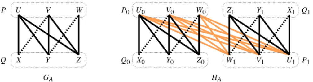
U V W X Y Z P Q P0 Q0 U0 V0 W0 X0 Y0 Z0 P1 Q1 Z1 Y1 X1 W1 V1 U1 GA HA
Fig. 1. Graphs GA and HA. A solid line between two sets implies that the two sets induce a complete bipartite graph, and a dotted line between two sets implies that there are some (but not all) edges between the two sets. Two color classes of HAare P0∪ Q1and Q0∪ P1.
3.2 Hardness for chain graphs
Next we prove the NP-hardness for chain graphs. Given an instance A of 3-Partition, we construct the graph GA = (P, Q; E). For convenience, let M = B + 3m − 4 and
γi = |{aj ∈ A | aj ≥ i}|. Note that 0 < γi ≤ 3m for m + 1 ≤ i ≤ a3m. In particular,
γm+1= 3m and γa3m > 0. First we define the vertex sets P = U∪V ∪W and Q = X∪Y ∪Z
as follows:
U= {ui| 1 ≤ i ≤ m}, V = {vi| m + 1 ≤ i ≤ a3m}, W = {wi| 1 ≤ i ≤ M − a3m}, X= {xi| 1 ≤ i ≤ 3m}, Y = {yi| m + 1 ≤ i ≤ a3m}, Z = {zi| 1 ≤ i ≤ M − a3m}. Next we define the edge set as follows:5
E= (X × U) ∪(Y× (U ∪ V))∪(Z× (U ∪ V ∪ W))
∪ {{xi, vj} | xi∈ X, m + 1 ≤ j ≤ ai}
∪ {{yi, wj} | yi∈ Y, 1 ≤ j ≤ M − a3m− γi}.
See Fig. 1 for a simplified illustration of GA.
Let G0and G1be two disjoint copies of GA. That is, GA ≃ G0 ≃ G1and V(G0)∩ V(G1)= ∅. By Pi, Qi, Ui, Vi, Wi, Xi, Yi, and Zi, we denote the vertex sets of Gi, i∈ {0, 1},
that correspond to the vertex sets P, Q, U, V, W, X, Y, and Z of GA, respectively.
Similarly, we denote the vertices of Gi, i∈ {0, 1}, that correspond to vertices uj, vj, wj,
xj, yj, and zjof GAby uij, v i j, w i j, x i j, y i j, and z i
j, respectively. We define the graph HAas
follows (see Fig. 1): V(HA)= V(G0)∪ V(G1) and E(HA)= E(G0)∪ E(G1)∪ (P0× P1).
Lemma 3.6. The graph HAis a chain graph.
Lemma 3.7. The degrees of vertices in HAsatisfy the following relations: degHA(u i j)= 2M+ 2m, degHA(vi j) = 2M − m + γj > 2M − m, 2M − a3m ≤ degHA(w i j) ≤ 2M − m, degHA(x i j) = ai, degHA(y i j) = M − γj < M, and degHA(z i j) = M. Moreover, ∆(HA) = 2M+ 2m and δ(HA)= a1. ⊓⊔
Now we prove that A is a yes instance of 3-Partition if and only if stc(HA)≤ k. We
divide the proof into two only-if part (Lemma 3.8) and if part (Lemma 3.9). Lemma 3.8. Let k= 3M − m − 2. If A is a yes instance, then stc(HA)≤ k.
Proof (Sketch). Let T be a spanning tree of HAwith the edge set as follows:
E(T )= {{u01, v} | v ∈ Q0∪ P1} ∪ {{u1j, x
1 h} | ah∈ Aj, 1 ≤ j ≤ m} ∪ {{u0j, x 0 j} | 2 ≤ j ≤ m} ∪ {{vi j, y i j} | i ∈ {0, 1}, m + 1 ≤ j ≤ a3m} ∪ {{wij, z i j} | i ∈ {0, 1}, 1 ≤ j ≤ M − a3m}.
Then, we can prove that cngHA(T )≤ k. ⊓⊔
Lemma 3.9. Let k= 3M − m − 2. If stc(HA)≤ k, then A is a yes instance.
4
Exponential-time exact algorithm
We have shown that STC is NP-complete even for very simple graphs. It is widely be-lieved that NP-hard problems cannot be solved in polynomial time. Thus we need fast exponential-time (or sub-exponential-time) algorithms for these problems. Nowadays, designing fast exponential-time exact algorithms becomes an important topic in theo-retical computer science. See a recent textbook of exponential-time exact algorithms by Fomin and Kratsch [8]. For STC, we can easily design an O∗(2m)- or O∗(nn)-time
algorithm that examine all spanning trees of input graphs, where n and m denote the number of vertices and the number of edges, respectively. In this section, we describe an algorithm for STC that runs in O∗(2n) time. Although it is still an exponential-time
algorithm, it is significantly faster than a naive algorithm.
Let G= (V, E) be a given undirected graph. For convenience, we denote |θG(X)| by
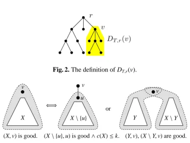
c(X). Note that c(∅) = c(V) = 0. Consider a spanning tree T with congestion at most k. We regard T as a rooted tree with root r ∈ V. We denote this rooted tree by (T, r). Let e = {u, v} ∈ E(T) be an edge of T, and without loss of generality, let u be the parent of v. Then, the congestion of e in T is equal to c(DT,r(v)), where DT,r(v) denotes the
set of descendants of v in (T, r). Since the congestion of T is at most k, we see that c(DT,r(v)) ≤ k. See Fig. 2. Conversely, if c(DT,r(v)) ≤ k for all v ∈ V \ {r}, then the
congestion of T is at most k. This is because there exists a one-to-one correspondence between the edges e of T and the vertices v in V\ {r} so that v is a deeper endpoint of e. We summarize this observation in the following lemma.
Lemma 4.1. The congestion of a rooted tree (T, r) is at most k if and only if c(DT,r(v))≤
k for every vertex v∈ V \ {r}. ⊓⊔
The lemma above suggests the following dynamic-programming approach. We call a pair (X, v) of a subset X ⊆ V and a vertex v < X a rooted subset of V. By definition, X, V for a rooted subset (X, v) of V. A rooted subset (X, v) of V is good if there exists a rooted spanning tree (T, v) of G[X ∪ {v}] such that c(DT,v(u))≤ k for all u ∈ X. Here, c
is a cut function of G, not of G[X∪ {v}]. By definition (X, v) is good when X = ∅. Note that there exists a rooted spanning tree (T, r) of G with congestion at most k if and only if the rooted set (V\ {r}, r) is good.
The following lemma provides a recursive formula that forms a basis of our algo-rithm (see Fig. 3).
r v
DT ,r(v)
Fig. 2. The definition of DT,r(v).
X
v u
X \ {u} v
(X,v) is good. (X \ {u},u) is good ∧ c(X) ≤ k. (Y,v), (X \ Y,v) are good. ⇐⇒
or
v
Y X \ Y
Fig. 3. An illustration of Lemma 4.2.
Lemma 4.2. Let (X, v) be a rooted subset of V with |X| ≥ 1. Then, (X, v) is good if and
only if at least one of the following holds.
1. There exists a vertex u∈ X ∩ NG(v) such that c(X)≤ k and (X \ {u}, u) is good.
2. There exists a non-empty proper subset Y⊆ X such that both of (Y, v), (X \ Y, v) are good.
Lemmas 4.1 and 4.2 above readily give an O∗(3n)-time dynamic programming
al-gorithm. However, the fast subset convolution method enables us to solve the problem in O∗(2n) time. We give a more detail below.
Let S be a finite set. For two functions f, g: 2S → R, their subset convolution is a
function f ∗ g: 2S → R defined as
( f ∗ g)(X) =∑
Y⊆X
f (Y)g(X\ Y)
for every X ⊆ S . Given f (X), g(X) for all X ⊆ S , we can compute ( f ∗ g)(X) for all X⊆ S in O∗(2n) total time, where n= |S | [1].
Back to the spanning tree congestion problem, let v∈ V be an arbitrary vertex. We define the function fv: 2V\{v} → R by the following recursion: fv(X) = 1 if X = ∅;
otherwise, fv(X)= ∑ u∈X∩NG(v) fu(X\ {u}) max{0, k − c(X) + 1} + ∑ ∅,Y(X fv(Y) fv(X\ Y),
where the empty sum is defined to be 0. It is easy to verify that fv(X) is non-negative
for every v∈ V and every X ⊆ V \ {v}.
The following lemma connects the functions fv, v∈ V and good rooted sets.
Lemma 4.3. Let (X, v) be a pair of a subset X ⊆ V \ {v} and a vertex v ∈ V. Then,
To apply the subset convolution method, we use the following functions. For each i∈ {0, 1, . . . , n − 1}, where n = |V|, and v ∈ V, let fi
v: 2V\{v}→ R be defined by
fvi(X)=fv(X) if|X| ≤ i, 0 if|X| > i, for all X⊆ V \ {v}. Then, it is not difficult to see the following.
1. For all v∈ X and X ⊆ V \ {v}, fn−1
v (X)= fv(X).
fvn−1(X)= fv(X).
2. For all v∈ V and X ⊆ V \ {v},
fv0(X)=
1 if X= ∅, 0 otherwise. 3. For all i∈ {1, . . . , n − 1}, v ∈ V, and X ⊆ V \ {v}
fvi(X)= ∑ u∈X∩NG(v) fui−1(X\ {u}) max{0, k − c(X) + 1} + ∑ ∅,Y(X fvi−1(Y) fvi−1(X\ Y) = ∑ u∈X∩NG(v) fui−1(X\ {u}) max{0, k − c(X) + 1} +∑ Y⊆X fvi−1(Y) f i−1 v (X\ Y) − 2 f i−1 v (∅) f i−1 v (X) = ∑ u∈X∩NG(v) fui−1(X\ {u}) max{0, k − c(X) + 1} + ( fi−1 v ∗ f i−1 v )(X)− 2 f i−1 v (∅) f i−1 v (X).
Our algorithm is based on these formulas. Step 1. For all v∈ V and X ⊆ V \ {v}, compute f0
v(X) based on the formulas above.
Step 2. For each i= 1, . . . , n − 1 in the ascending order, do the following. Step 2-1. For all v∈ V, compute the subset convolution fvi−1∗ fvi−1.
Step 2-2. For all v∈ V and all X ⊆ V \ {v}, compute fi
v(X) based on the formula
above. Step 3. If fn−1
v (V)> 0, then output Yes. Otherwise, output No.
The correctness is immediate from the discussion so far. The running time is O∗(2n)
since the running time of each step is bounded by O∗(2n). This is an algorithm for
solving the decision problem, but a simple binary search on k∈ {1, . . . , |E|} can provide the spanning tree congestion. Thus, we obtain the following theorem.
Theorem 4.4. The spanning tree congestion of a given undirected graph can be
Note that the algorithm also works for the weighted case with the O(n)-factor increase of the running time, since the number of distinct cut values c(X) is bounded by 2nand
so the binary search over the all possible values of c(X) takes at most O(log(2n))= O(n)
iterations. This is possible if we compute c(X) for all X ⊆ V beforehand, which only takes O∗(2n) time.
5
Remarks on cographs
We showed NP-completeness of STC for graphs of clique-width at most three. There-fore, it is quite natural to ask whether or not STC is NP-complete for graphs of clique-width at most two; that is, for cographs [7]. Although the complexity of STC for cographs remains unsettled, we have the following results.
Theorem 5.1. The spanning tree congestion of cographs can be approximated within
a factor four in polynomial time. Furthermore, the spanning tree congestion of chordal cographs can be determined in linear time.
References
1. A. Björklund, T. Husfeldt, P. Kaski, and M. Koivisto. Fourier meets Möbius: Fast subset convolution. In Proceedings of the 39th Annual ACM Symposium on Theory of Computing
(STOC ’07), pages 67–74, 2007.
2. H. L. Bodlaender, K. Kozawa, T. Matsushima, and Y. Otachi. Spanning tree congestion of
k-outerplanar graphs. In WAAC 2010, pages 34–39, 2010.
3. H.L. Bodlaender, F.V. Fomin, P.A. Golovach, Y. Otachi, and E.J. van Leeuwen. Parameter-ized complexity of the spanning tree congestion problem. submitted.
4. A. Brandstädt, V. B. Le, and J. P. Spinrad. Graph Classes: A Survey. SIAM, 1999. 5. A. Brandstädt and V. V. Lozin. On the linear structure and clique-width of bipartite
permu-tation graphs. Ars Combin., 67:273–281, 2003.
6. A. Castejón and M. I. Ostrovskii. Minimum congestion spanning trees of grids and discrete toruses. Discuss. Math. Graph Theory, 29:511–519, 2009.
7. B. Courcelle and S. Olariu. Upper bounds to the clique width of graphs. Discrete Appl.
Math., 101:77–114, 2000.
8. F. V. Fomin and D. Kratsch. Exact Exponential Algorithms. Springer, 2010.
9. M. R. Garey and D. S. Johnson. Computers and Intractability: A Guide to the Theory of
NP-Completeness. Freeman, 1979.
10. Martin C. Golumbic. Algorithmic Graph Theory and Perfect Graphs, volume 57 of Annals
of Discrete Mathematics. North Holland, second edition, 2004.
11. P. Hlinˇený, S. Oum, D. Seese, and G. Gottlob. Width parameters beyond tree-width and their applications. Comput. J., 51:326–362, 2008.
12. S. W. Hruska. On tree congestion of graphs. Discrete Math., 308:1801–1809, 2008. 13. K. Kozawa and Y. Otachi. Spanning tree congestion of rook’s graphs. Discuss. Math. Graph
Theory, to appear.
14. K. Kozawa, Y. Otachi, and K. Yamazaki. On spanning tree congestion of graphs. Discrete
Math., 309:4215–4224, 2009.
15. H.-F. Law. Spanning tree congestion of the hypercube. Discrete Math., 309:6644–6648, 2009.
16. H.-F. Law and M. I. Ostrovskii. Spanning tree congestion of some product graphs. Indian J.
Math., to appear.
17. C. Löwenstein, D. Rautenbach, and F. Regen. On spanning tree congestion. Discrete Math., 309:4653–4655, 2009.
18. M. I. Ostrovskii. Minimal congestion trees. Discrete Math., 285:219–226, 2004.
19. M. I. Ostrovskii. Minimum congestion spanning trees in planar graphs. Discrete Math., 310:1204–1209, 2010.
20. Y. Otachi, H. L. Bodlaender, and E. J. van Leeuwen. Complexity results for the spanning tree congestion problem. In WG 2010, volume 6410 of Lecture Notes in Comput. Sci., pages 3–14. Springer-Verlag, 2010.
21. S. Simonson. A variation on the min cut linear arrangement problem. Math. Syst. Theory, 20:235–252, 1987.
22. J.-H. Yan, J.-J. Chen, and G. J. Chang. Quasi-threshold graphs. Discrete Appl. Math., 69:247–255, 1996.
23. M. Yannakakis. Computing the minimum fill-in is NP-complete. SIAM J. Alg. Disc. Mech., 2:77–79, 1981.