Correlated anomalous diffusion: Random walk and Langevin equation

Correlated anomalous diffusion: Random walk and

Langevin equation

Kiyoshi Sogo,1,a兲 Yoshiaki Kishikawa,1Shuhei Ohnishi,2 Takenori Yamamoto,2Susumu Fujiwara,3and Keiko M. Aoki4

1_{Department of Physics, School of Science, Kitasato University, 1-15-1 Sagamihara,} Kanagawa 228-8555, Japan

2_{Faculty of Science, Toho University, 2-2-1 Miyama, Funabashi, Chiba 274-8510, Japan} 3_{Department of Macromolecular Science and Engineering, Graduate School of Science} and Technology, Kyoto Institute of Technology, Matsugasaki, Sakyo-ku, Kyoto 606-8585, Japan

4

Institute of Computational Fluid Dynamics, 1-16-5 Haramachi, Meguro- ku, Tokyo 152-0011, Japan

共Received 10 November 2009; accepted 11 January 2010; published online 11 March 2010兲 A random walk model is formulated and examined which gives the correlated anomalous diffusion found in molecular dynamics simulations. The mean square displacement共MSD兲 shows a logarithmic behavior in one dimension. Correspond-ing Langevin equation is constructed by solvCorrespond-ing the inverse problem which gives a procedure to derive random impulse correlation from MSD function. © 2010 American Institute of Physics. 关doi:10.1063/1.3309329兴

I. INTRODUCTION

Recently a new molecular dynamics 共MD兲 method was introduced by one of the authors 共Aoki1_{兲. This MD method, which utilizes a symplectic integrator, has an advantage that all the} thermodynamic states are obtained through constant pressure and constant temperature processes and can even produce nonequilibrium steady states including some glass states.

Such a method was applied to the study of single-component soft-core repulsive particle system.2Some features and results of Ref.2 are summarized as follows.

共1兲 A soft-core potential of finite radius is used with only repulsive part of Lennard-Jones-type potential.

共2兲 Simulation scheme employed is that of the Nosé–Poincaré Hamiltonian.

共3兲 Symplectic method is used to integrate the equations of motion with constant pressure and constant temperature.

共4兲 Three branches of nonequilibrium steady states are found. They are shown in the phase diagram Fig.1, where共a兲, 共b兲, and 共c兲 are the newly found glass states, while 共d兲 is the solid phase and共e兲 is the liquid phase.

共5兲 The properties of these states are analyzed in detail, such as specific volume, lattice structure, mean square displacement 共MSD兲, and dynamical distribution functions 共van Hove self-correlation function兲.

These results show some of the specific properties of glass state: the dynamical heterogene-ities and the intermittent diffusivity. Especially in the obtained movies particles are observed to stay on the preconstructed lattice sites for a mean time, and suddenly jump onto the neighboring sites, showing a behavior of anomalous diffusion.

Anomalous diffusion observed in such single-component soft spherical particles MD could be

a兲_{Electronic mail: [email protected].}

51, 033302-1

examined by two models. The purpose of the present paper is to construct a random walk model simulating such anomalous diffusion and to analyze a Langevin equation model corresponding to it.

The first one is to construct a stochastic model, which will be discussed in Sec. II. Since particles move in a correlated manner each other, let us call this stochastic model the correlated diffusion model. The second model is to consider a Langevin equation which imitates a correlation effect and to solve such equation, which will be discussed in Sec. III.

II. RANDOM WALK MODEL OF ANOMALOUS DIFFUSION A. Stochastic model of correlated diffusion

The model considered here is composed of many particles on a regular lattice 共each site is empty or occupied by one particle兲. Additionally, the system proceeds under stochastic dynamics with the following rules.

共1兲 Particle always jumps to the neighboring site if it is empty.

共2兲 If there are many sites to jump, it chooses one of them with an equal probability. 共3兲 The order of jumps for particles is determined randomly for the molecular democracy.

In the simulations the algorithm called MERSENNE TWISTER 共MT19937兲 of GNU Scientific

Library共GSL兲 is used to generate quasirandom numbers. B. Results of simulations

1. One dimensional case

While numerical simulations, the MSD function M共t兲 and the van Hove functions F共k,t兲 are computed. These quantities are defined as follows:

M共t兲 =

冓

兺

冔

冓

兺

冔

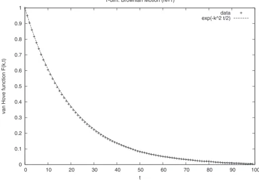
where具¯典 implies the sample average. The number of sampling is taken as 105typically. For the particle number N = 1 case, the problem can be analyzed rigorously, since the prob-ability distribution function P共x,t兲 obeys the difference equation

0.235 0.24 0.245 0.25 0.255 0.26 0.265 0.27 80 100 120 140 160 180 200 Volume/N Temperature (a) (b) (c) (d) (e)

FIG. 1. 共Color online兲 The phase diagram for the large 共N=2048兲 system. Nonequilibrium steady states identified as the glass states are found关共a兲–共c兲兴.

P共x,t + 1兲 =1₂共P共x + 1,t兲 + P共x − 1,t兲兲, 共2.3兲 which can be solved exactly. For example, the MSD function is given by

M共t兲 = 具共x共t兲 − x共0兲兲2典 = t, 共2.4兲

and the van Hove function F共k,t兲 is computed as F共k,t兲 = exp

冉

2

2t

冊

Figure 2 shows the van Hove function F共k,t兲 for N=1 and the theoretical result 共2.5兲. The agreement is very well.

As the particle number N increases, the van Hove function F共k,t兲 decays slowly as shown in Fig.3.

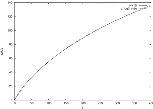
The decay property of F共k,t兲 is not exponential but power law such as t−␥for large t. This can be more directly understood by observing MSD, which is shown in Fig.4. Since the motion of a particle is interrupted by other particles, the MSD becomes smaller than that of N = 1.

Since the behavior of MSD in Fig.4 as a function of t is estimated as

M共t兲 =

再

␤t 共t Ⰶ t0兲,

冎

共2.6兲 with some t₀, the numerical results can be fitted by an interpolating function,

M共t兲 = a log

冉

冊

1-dim. Brownian Motion (N=1)

data exp(-k^2 t/2)

=

再

共a/b兲t 共t Ⰶ b兲,

冎

which is shown in Fig.5. 0 0.1 0.2 0.3 0.4 0.5 0.6 0.7 0.8 0.9 1 0 10 20 30 40 50 60 70 80 90 100 van Hove function F(k,t) t N= 1 N=10 N=20 N=30

FIG. 3. The van Hove functions F共k,t兲 of k=␲/10 for several particle numbers N.

0 50 100 150 200 250 300 350 400 0 50 100 150 200 250 300 350 400 MSD t N= 1 N= 5 N=10 N=20

The coefficient a of fitting function a log共1+t/b兲 is shown for several values of the concen-tration c = N/L 共L=the number of sites兲 in Fig. 6, where the data are fitted well by the curve a =␤·共1−c兲/c with ␤= 10.2602.

Now the van Hove function F共k,t兲 is, in general, related with M共t兲 as follows: 0 20 40 60 80 100 120 140 0 50 100 150 200 250 300 350 400 M S D t N=10 a*log(1+t/b)

FIG. 5. Numerical results can be fitted by the function a log共1+t/b兲.

0 10 20 30 40 50 60 70 80 90 100 0.1 0.2 0.3 0.4 0.5 0.6 0.7 0.8 0.9 1 a c a b*(1-c)/c

FIG. 6. Coefficient a of M共t兲=a log共1+t/b兲 vs the concentration c=N/L. The data can be fitted well by the curve a =␤·共1−c兲/c with␤= 10.2602.

F共k,t兲 = 具exp共ik共x共t兲 − x共0兲兲兲典 = exp

冉

冊

冉

冊

Whether the process is Gaussian or not can be examined by checking whether the kurtosis defined by kurtosis =m4 m22 = 具共x共t兲 − x共0兲兲 4_典 具共x共t兲 − x共0兲兲2_典2 共2.10兲

is equal to 3 or not. Since typical value of this quantity is 3.0933¯, for N=10, for example, our model can be considered as a Gaussian random process. In fact, the both sides of Eq.共2.9兲agree well when we use the numerical results for both quantities. The van Hove function F共k,t兲 decays as t−␥when M共t兲 behaves as␣log t for large t, where the power is given by␥=共k2_/2兲·␣.

2. Two dimensional case

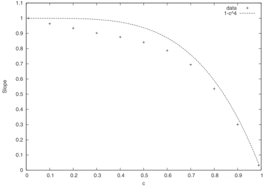
In two dimensional case the MSD function obtained is, surprisingly, different from that of one dimensional case. It has t linear behavior, as shown in Fig.7. As before, the case of N = 1 gives the rigorous M共t兲=t result as expected. Moreover, the slope decreases as the particle number N increases, which is a natural behavior due to mutual interruptions. The reason for this dimension-ality dependent difference may be interpreted such that a particle in two dimensions can go around the other particles to diffuse.

Let us consider here a simple mean field theory by constructing an approximate Fokker– Planck equation. We set the particle number N, the number of sites L2_{, and the particle} concen-tration c = N/L2_{, then the probability q that four neighboring sites are all occupied is estimated as} q = c4_{. Then we have} 0 100 200 300 400 500 600 700 800 900 1000 0 100 200 300 400 500 600 700 800 900 1000 MSD t MSD on 2-dim. 10x10 lattice N= 1 N=10 N=50 N=90

P共x,y,t + 1兲 = p · 共P共x + 1,y,t兲 + P共x − 1,y,t兲 + P共x,y + 1,t兲 + P共x,y − 1,t兲兲 + q · P共x,y,t兲, 共2.11兲 where the probability p =共1−q兲/4. Then after some calculations we have

M共t兲 ⬅ 具共x共t兲 − x共0兲兲2+共y共t兲 − y共0兲兲2典 = 共1 − c4兲 · t, 共c = N/L2兲. 共2.12兲 This formula is compared with the simulations in Fig.8, and the agreement is rather good.

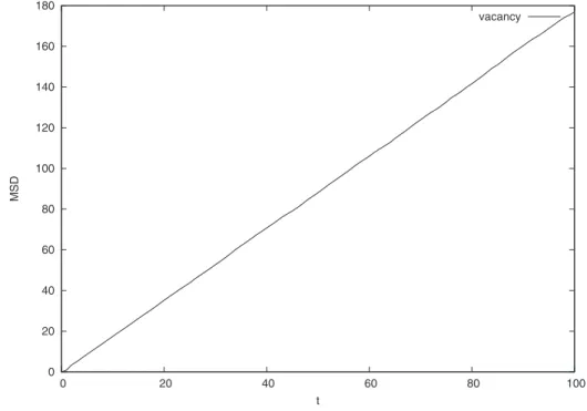
C. Diffusion of a vacancy

It may be interesting to consider the case that the number of particles is less than the number of sites by 1. Then our model can be viewed as a diffusion of a vacancy. The result is given in Fig. 9, which shows an ordinary Brownian motion but with a larger slope. This is because that the vacancy can move to farther positions in a single time step.

III. LANGEVIN EQUATION FOR ANOMALOUS DIFFUSION

The random walk model discussed in Sec. II suggests that there might be an analytical theory by Langevin equation method. Let us consider a Langevin equation for single particle for which unknown random impulse is applied. In other words, we suppose that the correlated force from other particles can be treated to produce such random impulse. Moreover, we ask ourselves what kind of impulse correlation can give the observed MSD property. We formulate below such question as an inverse problem of MSD and solve the derived equation for several cases.

A. Langevin equation and inverse problem of MSD Let us consider a Langevin equation

0 0.1 0.2 0.3 0.4 0.5 0.6 0.7 0.8 0.9 1 1.1 0 0.1 0.2 0.3 0.4 0.5 0.6 0.7 0.8 0.9 1 S lope c data 1-c^4

dx

dt= f共t兲, 共3.1兲

where the random function f共t兲, a velocity produced by random impulsive force, is assumed to be a Gaussian process with

具f共t兲典 = 0, 具f共t兲f共t

⬘

⬘

The impulse correlation␺共t兲 is assumed to be an even function:␺共−t兲=␺共t兲. Since the differential equation 共3.1兲is integrated as

x共t兲 = x共0兲 +

冕

t

f共t

⬘

⬘

M共t兲 = 具共x共t兲 − x共0兲兲2典 =

冕

冕

冕

冕

冕

冕

M共t兲 = 2

冕

冕

0 20 40 60 80 100 120 140 160 180 0 20 40 60 80 100 M S D t vacancy

⌽共t兲 = L−1

冉

s·␺ˆ 共s兲

冊

Therefore, the derivative of MSD function is given by

M˙ 共t兲 = 2⌽共t兲 = 2L−1

冉

s ·␺ˆ 共s兲

冊

冉

s·L共␺共t兲兲

冊

which gives the MSD function M共t兲 from the random impulse correlation function␺共t兲. Let us call this the proper problem of MSD.

For example, if ␺共t兲=e−␥兩t兩, we have for t⬎0 M˙ 共t兲 = 2L−1

冉

冊

冉

冊

␺共t兲 =1

2L−1共s · L共M˙共t兲兲兲, 共3.8兲

which we call the inverse problem of MSD to derive the impulse correlation ␺共t兲 from MSD function M共t兲.

B. Solution of the inverse problem

Let us consider solutions of inverse problem for some typical MSD functions. The case of M共t兲=t . This is the case of ordinary Brownian motion,

␺共t兲 =1

2L−1共s · L共M˙共t兲兲兲 = 1

2L−1共s · L共1兲兲 =␦共t兲, 共3.9兲

where we usedL共1兲=1/s and L−1_共1兲=2␦_{共t兲. This is the well known result.} The case of M共t兲=t␣ . This is the case of fractional diffusion,3

␺共t兲 =1 2L −1_{共s · L共M˙共t兲兲兲 =}␣ 2L −1_{共s · L共t}␣−1_{兲兲 =}1 2⌫共␣+ 1兲L −1

冉

冊

L共t␤−1_{兲 = ⌫共␤兲 ·} 1

s␤ 共␤⬎ 0兲, 共3.11兲

and its inverse formula is used. In the above result the parameter␣should satisfy 1⬍␣⬍2 by the physical requirement that the correlation␺共t兲 decays when t→⬁. The limit␣= 1 is the previous case.

The case of M共t兲=log共1+t/␶兲 . This is the case of logarithmic MSD function observed in the previous section,

M共t兲 = log

冉

␶

冊

⌽共t兲 =1 2M˙ 共t兲 = 1 2· 1 t +␶, 共3.13兲 we have ␺共t兲 =1 2L −1

冉

冉

冊冊

冉

冊

which have a long range negative correlation. However, it should be noted that this␺共t兲 satisfies

冕

⬁

␺共t兲dt = 0. 共3.15兲

If the sign of such integration is negative, the system shows unphysical behavior: it does not diffuse. All physical diffusion processes should have non-negative values.4Above result 共3.15兲 implies that our logarithmic MSD is indeed the marginal case.

IV. SUMMARY AND DISCUSSION

A stochastic model of the correlated diffusion is introduced and analyzed. By numerical simulations the MSD and the van Hove self-correlation functions are computed. Their behaviors for one dimensional case are similar to those observed in the glass phase of our MD simulations. Then the inverse problem of Langevin equation is studied so that the random impulse correlation function is determined to provide the given MSD behavior. Especially the impulse correlation is determined which gives the logarithmic MSD function found in the simulations.

As far we have considered for brevity the simplest Langevin equation. Moreover, the anoma-lous diffusion has been attributed to the long range impulse correlation. We may, however, extend the Langevin equation to more general ones. For example, one may consider equations for the velocityv共t兲 with a memory term5–7

dv dt +

冕

t

␸共t − t

⬘

⬘

⬘

Or one may even consider a Langevin equation with a fractional derivative.3 Furthermore, the intermittent diffusion observed in the MD simulation might be explained by considering a waiting time probability discussed by Scher and Montroll.8Such possibilities will be discussed in future works.

ACKNOWLEDGMENTS

The authors wish to thank the anonymous referee for enlightening comments, especially on the implication of 共3.15兲, on the possibility to explain the intermittency by the waiting time distribution, and for reminding them some references.

1_{K. M. Aoki,J. Phys. Soc. Jpn.77, 044003共2008兲.}

2_{T. Yamamoto, S. Fujiwara, K.M. Aoki, K. Sogo and S. Ohnishi, “Glassy dynamics in non-equilibrium steady states of}

single-component systems,” J. Phys. Soc. Jpn.共submitted兲.

3_{B. J. West, M. Bologna, and P. Grigolini, Physics of Fractal Operators共Springer, New York, 2003兲.} 4_{R. Cakir, P. Grigolini, and A. A. Krokhin,Phys. Rev. E74, 021108共2006兲.}

5_{H. Mori,Prog. Theor. Phys.33, 423共1965兲;Prog. Theor. Phys.34, 399共1965兲.} 6_{J. M. Porrà, K.-G. Wang, and J. Masoliver,Phys. Rev. E53, 5872共1996兲.} 7_{R. Cakir, P. Grigolini, and A. A. Krokhin,Chaos, Solitons Fractals34, 19共2007兲.} 8_{H. Scher and E. W. Montroll,Phys. Rev. B12, 2455共1975兲.}