A Heuristic Rule Reduction Approach to Software Fault-proneness Prediction
11
0
0
全文
(2) A Heuristic Rule Reduction Approach to Software Fault-proneness Prediction Akito Monden* Jacky Keung† Shuji Morisaki‡ Yasutaka Kamei+ Ken-ichi Matsumoto* *Graduate School of Information Science, Nara Institute of Science and Technology 8916-5 Takayama, Ikoma, Nara 630-0192, Japan †. Department of Computing, Hong Kong Polytechnic University Hung Hom, Kowloon, Hong Kong ‡. Faculty of Informatics, Shizuoka University 3-5-1 Shirokita, Naka-ku, Hamamatsu, Shizuoka 432-8011, Japan +. Graduate School and Faculty of Information Science and Electrical Engineering, Kyushu University West 2-810, 744 Motooka, Nishi-ku, Fukuoka 819-0395 Japan *{akito-m, matumoto}@is.naist.jp, †[email protected], ‡[email protected], + [email protected]. Abstract— Background: Association rules are more comprehensive and understandable than fault-prone module predictors (such as logistic regression model, random forest and support vector machine). One of the challenges is that there are usually too many similar rules to be extracted by the rule mining. Aim: This paper proposes a rule reduction technique that can eliminate complex (long) and/or similar rules without sacrificing the prediction performance as much as possible. Method: The notion of the method is to removing long and similar rules unless their confidence level as a heuristic is high enough than shorter rules. For example, it starts with selecting rules with shortest length (length=1), and then it continues through the 2nd shortest rules selection (length=2) based on the current confidence level, this process is repeated on the selection for longer rules until no rules are worth included. Result: An empirical experiment has been conducted with the Mylyn and Eclipse PDE datasets. The result of the Mylyn dataset showed the proposed method was able to reduce the number of rules from 1347 down to 13, while the delta of the prediction performance was only .015 (from .757 down to .742) in terms of the F1 prediction criteria. In the experiment with Eclipsed PDE dataset, the proposed method reduced the number of rules from 398 to 12, while the prediction performance even improved (from .426 to .441.) Conclusion: The novel technique introduced resolves the rule explosion problem in association rule mining for software proneness prediction, which is significant and provides better understanding of the causes of faulty modules.. Keywords-defect prediction; empirical study; association rule mining; data mining; software quality. I.. INTRODUCTION. According to Pareto's law that 80 percent of the faults can be found in 20 percent of the modules, identification of fault-prone modules is an important challenge for effective testing and/or software inspection [11][13] [18]. To date, various multivariatemodeling techniques applicable to fault-prone module prediction have been used, including the most commonly used linear discriminant analysis [18], logistic regression analysis [16], classification tree [9], support vector machine[6] and random forest [10]. However, the problem common to all these prediction models is that the model itself is not easily understandable to human, that is, software engineers cannot easily recognize and agree as why a certain module is faulty (or not faulty.) Even a simplest linear discriminant model, correlations between predictor variables makes it difficult to interpret their coefficients clearly. In addition, such difficulties can be easily interpreted as a negative opinion: “this technique (or model) does not fit to our project”, which is commonly uttered by engineers who do not wish to use any newer techniques in their project. This paper’s primary focus is on the association rule mining described in [1][22], which are much more understandable since rules are described in a simple and intuitive form (condition faulty) or (condition not faulty). For example, a rule “(20 < cyclomatic number) and (10 < fan-in) fault prone” implies and indicates that a module is faulty if its cyclomatic number is larger than 20 and its fan-in is larger than 10. When such rules were derived from a past project’s module dataset, we could use them for the prediction of an ongoing or a future planned project. However, as we will explain in Section II.D, association rule mining suffers from a rule explosion problem which also makes human understanding difficult, i.e. there are too many similar rules and/or complex rules are mined. In our study, the Mylyn data set (consists of 13 metrics of 1023 modules) produced 1346 rules even though we only have mined the high confidence (≥0.75) rules (see Section V). We could reduce these rules by.
(3) commonly used rule measures such as confidence and support, but using these measures cannot reduce similar rules or complex rules. Instead of using these measures, we could remove complex rules by mining simple rules only (whose antecedents are short); but in this case we may sacrifice the prediction accuracy. Based on the above discussion, this study attempts to balance the following two requirements: (Req.1) Remove similar and/or complex rules as much as possible from a rule set. (Req.2) At the same time, not sacrificing the prediction performance. To achieve these requirements simultaneously, we propose a new algorithm for rule reduction. The notion of this algorithm is to reduce long (complex) rules as much as possible unless their confidence is enough higher than similar shorter rules. We will show the effectiveness of the algorithm using the Mylyn and Eclipse PDE datasets in our experiment. The next section introduces association rule mining and its rule explosion problem. Followed by Section III, in which we propose an algorithm for rule reduction. Section IV describes an experiment setting to evaluate the algorithm and Section V describes the result and discussion of the experiment. We summarize this paper and presents future research directions in Section VI.. II.. BACKGROUND: RULE MINING AND ITS EXPLOSION PROBLEM. Association rule mining is a typical method for discovering the patterns of co-occurrences of the attributes in a dataset. Below we introduce its details, related work and the rule explosion problem.. A.. Association Rule Mining. Association rule mining is also referred to as an association analysis. Its applications have been applied to discover associations hidden amongst data in the POS (Point-Of-Sales) product-purchasing logs of retail stores [1], access logs of website [25], proteins [19], etc. In the case of POS logs, researchers have mined rules about products purchased together, such as “(purchases product A)∩(purchases product B) purchases product C.” There are a number of possible ways to use such rules, for example a retailer could place products A, B, and C near to each other in the store so that customers can find them easily; or, it could ensure revenues by setting the prices of antecedent products A and B to make up the discounts on the sale price of consequent product C. Association rule mining (association analysis) is defined by Agrawal et al. as follows [1]. Let I = {I1, I2, ..., Im} be a set of items where each Ik (1 ≤ k ≤ m) is an item and m is the number of unique items. An association rule is denoted by an expression A B, where A I, B I, B ∉ A. We refer to A as the antecedent of the rule, and B as the consequent of the rule. Let a database D be {T1, T2, ..., Tn} where Ti I is called a transaction, n is the number of transactions. We call “Ti satisfies the rule A B” if A Ti B Ti holds. In the POS log example, D corresponds to a log of all past purchases and Ti D corresponds to one purchase by a customer. I corresponds to all unique products sold. A I corresponds to. one or more products purchased. B I corresponds to a product purchased together with A. In this paper, the antecedent expresses a condition of module metrics and the consequent denotes either a module is faulty (i.e. a module contains one or more fault) or not faulty (i.e. a module contains no fault). The association analysis is normally applied to qualitative variables (ordinal scale variables); ratio scale and interval scale variables are generally pre-processed and transformed to ordinal scale variables before rule mining. For example, it would be possible to transform “cyclomatic number” and “fan-in” into ordinal scale variables consisting of three categories — low [0, 10), medium [10, 30) and high [30, ∞ ). A rule “(cyclomatic number = medium)∩(fan-in = high) faulty” indicates that a module is fault-prone if its cyclomatic number is between 10 and 30, and its fan-in is larger than or equal to 30. There are two key measures of interestingness (or importance) of a rule as follows. Support: Support is an indicator of rule frequency. It is expressed as support(A B), which is equal to a/n, where a = |{T D|A T B T}| and n = |D|. Confidence: Confidence is the probability that consequent B will follow antecedent A. It is expressed as confidence(A B), which is equal to a/b, where a is defined as in Support and b = |{T D|A T}|. For example, assuming that the number of modules expressed as n = 20, the number of modules that satisfies A is 10, the number of modules that satisfies B is 8, and the number of modules that satisfies both A and B is 6. For the rule A B, the support is .3 (= 6/20), the confidence is .6 (= 6/10). We also define the length of a rule as follows: Length: Length is an indicator of rule’s complexity (larger length indicates more complex rules). It is expressed as length (A B), which is equal to the number of items in A. For example, the length of the rule “(cyclomatic number = medium)∩(fan-in = high) faulty” is 2 since two metrics (cyclomatic number and fan-in) is in the antecedent. Finally, we define the relationship between two rules as follows: Subsumed: We call that a rule A B subsumes a rule C B if C A. For example, a rule “(cyclomatic number = medium) faulty” subsumes a longer rule “(cyclomatic number = medium)∩(fan-in = high) faulty.”. B.. Fault-prone Module Prediction by Rules. A rule set obtained by association rule mining is often used as predictive rules for the future business. In general, higher confidence (or support) rules yield higher prediction accuracy; thus, after rules are mined from module metrics and fault data sets, a set of rules whose confidence (or support) is greater than their threshold confidence (or support) are selected and used for their prediction. To conduct a prediction, given a selected rule set and a target module to be predicted, we need to consider that more than one rules can match the module, that is, module metrics satisfy the antecedent means of multiple rules. This becomes a problem when.
(4) matched rules had different consequents (faulty and not-faulty). A typical way to handle this situation is to classify the module by the majority of rules’ consequent [7]. Another way is to select the longest rules among matched rules [22].. (P3) Some rules are very long. Usually long rules are difficult to interpret by human. For example, “α∩β∩γ∩δ∩ε∩λ∩ζ faulty” is too complex to understand. Moreover, very long rules can cause overfitting problem.. We also need to consider the cases where no rule matches the module. In such cases, Kamei et al. proposed to conduct a modelbased prediction as a complementary method [7].. There are several possible ways to reduce the rules. A typical practice is to select high confidence (or support) rules. For example, suppose we have the following four rules and confidence values:. This paper employs a novel approach to prediction. To keep the rule set small and understandable, we mined rules whose consequent is “faulty” only, where non-faulty rules are ignored. If one or more rules match the module, then we consider it is faulty. Otherwise, we classify it as non-faulty. By selecting high confidence (and support) rules, we could also obtain promising prediction accuracy with “faulty” rules only (see Section V.). C.. Related Work: Rule Mining in Software Engineering. A number of cases studied have reported association rule mining for a software related dataset. Kamei et al. proposed a hybrid faulty module prediction method combining association rule mining with a model based approach (logistic regression analysis) for the purpose of improving the performance of fault-prone module prediction [7]. Song et al. [22] mined association rules from defect data logged during development (type of defect cause, correction effort, etc.) to predict types of defects that would occur simultaneously and to predict defect-correction effort (staff-hours: “one hour or less”, “one hour to one day”, “one day to three days”, and “more than three days”). Hamano et al. [5] collected risk evaluation metrics in software development, and conducted association analysis to reveal project-confusion factors (whether development budgets or deadline standards will be overrun). Michail [12] found reuse patterns of libraries in application software by using association rule mining, and tried to use the derived patterns in building a class library. Morisaki et al. [14] proposed an extended association rule mining method that takes advantage of interval and ratio scale variables, instead of simply replacing them into nominal or ordinal variables. In the proposed method, an extended rule describes the statistical characteristic of quantitative variables (e.g. mean and standard deviation) in the consequent part together with related metrics (e.g. “lift of mean” and “lift of standard deviation”) so that conditions producing distinctive statistics can be discovered as rules. They also conducted an empirical study to reveal rules associated with defect correction effort of an industry project. However, none of these studies focused on reducing the rule set to solve the rule explosion problem, which we will explain in the next subsection.. D.. Rule Explosion Problem. “Rule explosion” effect refers to the fact that an excessive number of rules are generated by the association rule mining technique. This causes the following problems for human understanding. (P1) Similar rules are included in the derived rule set. For example, we may have a slightly different two rules “α∩β∩γ∩δ faulty” and “α∩β∩γ∩ε faulty” in the rule set. This makes it difficult for an engineer to decide which rule should be focused on. (P2) Some rules subsumes other rules. For example, “α∩β faulty” subsumes “α∩β∩γ faulty”. From the point of view of prediction, the latter rule is not needed.. (Rule #1) α∩β faulty (Rule #2) α∩β∩γ faulty (Rule #3) α∩λ∩ε faulty (Rule #4) λ∩ζ faulty. Confidence=82% Confidence=83% Confidence=92% Confidence=30%. In this case, rule #4 can be removed by setting a threshold value (e.g. minimum confidence = 70%) in rule selection. However, rules #1,2,3 still remain, thus we cannot solve neither of the problems P1, P2 and P3 above. We could also reduce the rules by setting the threshold values to the length of rules (e.g. maximum length = 2.) In this case, rules #2 and #3 are removed; however, the rule #3 should not be removed because it has very high confidence (92%). We need to consider that some long rules are worth selecting if they have high indication of confidence, i.e. they are likely to increase the prediction accuracy. On the contrary, we could reduce the rules by selecting long rules rather than short rules since selecting longer rules is one of the promising practices in rule-based prediction [22]. By this approach, problem P2 may be solved, but P1 and P3 cannot be solved. In addition, we need to consider that not all the longer rules are worth selecting than the shorter rules, as we will explain in the next section.. III. PROPOSED METHOD A.. Basic Idea. Given a rule set, our goal is to remove as many rules that are (1) similar to others, (2) subsumed by other rules or (3) complex (i.e. long), while not losing the prediction performance of the rule set. Our basic idea is to evaluate the tradeoffs between length and confidence of a rule. We remove rules unless they have enough confidence for their length. Suppose we have the following two rules in the derived rule set. (Rule #1) α∩β faulty (Rule #2) α∩λ∩γ faulty. Confidence=82% Confidence=83%. In this case, rule #2 is longer (i.e. more difficult to understand) than rule #1. We consider that rule #2 is NOT worth selected because it could gain only 1% improvement (in confidence) by increasing the length. Since the longer rules are more difficult to understand, we do not select longer rules unless it yields acceptable improvements in confidence, as shown in the following example: (Rule #1) α∩β faulty (Rule #2) α∩λ∩ε faulty. Confidence=82% Confidence=92%. In this case, we consider that rule #2 is worth selecting because enough improvement (10% in confidence) is achieved. If we remove rule #2, then we might lose the prediction accuracy. To.
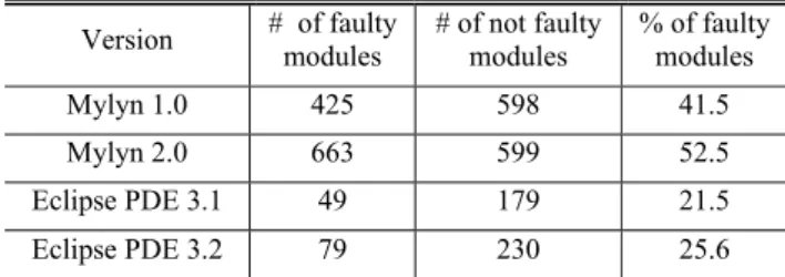
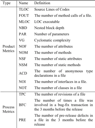
(5) 1: Let Rx be a set of rules whose length = x in the input rule set R 2: Let x = (length of the shortest rule in R) 3: Let R’ = Rx // keep all the shortest rules in the reduced rule set 4: Loop: 5: Let x = x + 1 6: Let confidence = confidence + improvement // set a threshold for length = x rules 7: if Rx = then goto End 8: For each rule r in Rx { // start inspecting longer rules whether they are worth selected 9: if r is subsumed by one of rules in R’ then remove r from Rx 10: if confidence(r) < confidence then remove r from Rx 11: } 12: Let R’ = R’∪Rx // add selected rules to the reduced rule set 13: goto Loop: 14: End: return R’ // return the reduced rule set Figure 1. Rule reduction algorithm decide whether a rule is worth selecting or not, this paper employs a threshold improvement to the improvement of rule’s confidence.. Table I. Statistical summary of Mylyn and Eclipse PDE data sets. A yet another case is that a shorter rule subsumes a longer rule as follows. (Rule #1) α∩β faulty (Rule #2) α∩β∩ε faulty. Confidence=82% Confidence=93%. In this case, rule #2 could be selected since it has high confidence level. However, if we decided to select rule #1, then rule #2 must be removed as it is subsumed by rule #1.. B.. Rule Reduction Algorithm. After mining a set of rules from a module data set with threshold values of minimum support and confidence, our rule reduction algorithm starts with selecting all the shortest (e.g. length = 1) rules. Then, we look through the 2nd shortest rules (length = 2) if there exists good enough rules to be selected in comparison with already selected shorter rules based on the threshold improvement. We also remove rules that are subsumed by shorter rules. We continue this selection for longer rules (length = 3, 4, …) until no rules are worth selected. ∪ ∪ ⋯∪ be a rule set derived by Let R={ association rule mining with threshold values: minimum support = support minimum confidence = confidence where Rx be a set of rules whose length = x. Then, Fig. 1 shows our rule reduction algorithm that removes rules from R and obtains a reduced rule set R’. To explain how the algorithm works, here we assume that initial threshold values are confidence = 0.75 and improvement = 0.05, and the given rule set R consists of the following rules. (Rule #1) α faulty Confidence=75% (Rule #2) β faulty Confidence=76% Confidence=82% (Rule #3) α∩λ faulty (Rule #4) λ∩ζ faulty Confidence=74% (Rule #5) λ∩γ faulty Confidence=80% In line 1 of Fig.1, we will have two rule subsets as follows. R1 = {Rule #1, Rule #2} R2 = {Rule #3, Rule #4, Rule #5} Next, in line 2 and 3, we will have x = 1 and R’ = R1 = {Rule #1, Rule #2}. Then, we start inspecting length = 2 rules in R2 whether they are worth selected or not. In line 6, we set a new threshold. Version. # of faulty modules. # of not faulty modules. % of faulty modules. Mylyn 1.0. 425. 598. 41.5. Mylyn 2.0. 663. 599. 52.5. Eclipse PDE 3.1. 49. 179. 21.5. Eclipse PDE 3.2. 79. 230. 25.6. confidence = 0.8 for length = 2 rules. In line 8, in the first iteration, we pick r = Rule #3, and in line 9, it is removed from R2 because it is subsumed by Rule #1 in R’. Then we go back to line 8 for the second iteration, and r = Rule #4 this time. In line 10, since confidence(Rule #4) < 0.8, Rule #4 is not considered worth selecting, so it is removed from R2. Next, for the third iteration in line 8, we have r = Rule #5. Since Rule #5 is not subsumed by any of rules in R’ and also confidence(Rule #5) 0.8, it is kept in R2. Then in line 12, new R’ becomes {Rule #1, Rule #2, Rule #5}, and we will go back to Loop in line 4. Finally, in line 6, since R3 is empty, i.e. there is no length=3 rules in R, we goto line 14.. IV. EXPERIMENTAL SETTING To evaluate the true effectiveness of the proposed method, we compare our method with a commonly used rule selection method that sets a threshold in confidence. The following describes datasets, evaluation criteria and procedures used in the experiment.. A.. Target Software. In this experiment, we collected module (i.e., source file) datasets from two versions in Mylyn [3] and Eclipse PDE [4] both written in Java. Table I summarizes the statistics of the used datasets. Mylyn dataset has a good balance of faulty and not faulty modules while Eclipse PDE is class-imbalance data (21.5% faulty modules in v3.1).. B.. Used Metrics. In Mylyn dataset, we measured both product metrics and process metrics (Table II). For product metrics, we used Understand [24] to extract complexity and size metrics for each of the files. For process metrics, we used the metrics proposed by Moser et al. [15][21]. To measure the process metrics, we used CVS repository provided by Eclipse Foundation..
(6) Table III. Additional Metrics in Eclipse PDE dataset. Table II. Measured Metrics in Mylyn dataset Type. Product Metrics. Process Metrics. Type. Name. Definition. Source Lines of Codes. CBO. Coupling Between Object classes. FOUT. The number of method calls of a file.. Number Of Children of a class. MLOC. LOC executable. Product Metrics. NOC. Name. Definition. TLOC. NBD. Nested block depth. PAR. Number of parameters. VG. Cyclomatic complexity. NOF. The number of attributes. NOM. The number of methods. DIT. Depth of Inheritance Tree. LCOM. Lack of Cohesion in Methods. Table IV. Characteristics of the initial rule set (Mylyn) Rule length. Average support. NSF. The number of static attributes. 1. NSM. The number of static methods. 2. 8. .797. .139. ACD. The number of anonymous type declarations in a file. 3. 84. .811. .068. NOI. The number of interfaces in a file.. 4. 397. .819. .040. NOT. The number of classes in a file. 5. 858. .825. .031. TPC. The number of revisions of a file. 1347. .822. .037. BFC. The number of times a file was involved in a bug-fix transaction in the 3 months before the release. PRE. The number of pre-release defects in a file in the 3 months before the release. all. In Eclipse PDE dataset, we measured object oriented metrics (Table III) in addition to metrics of Mylyn dataset.. Recovery of Bugs. We obtained the number of bugs in source code files using the SZZ algorithm [23]. This algorithm identifies when a bug was injected into the code and who injected it by linking a version archive (such as CVS) to a bug database (such as Bugzilla).. D. Initial Rule Set We used NEEDLE [14] as an association rule miner. To obtain an initial rule set (for applying rule reduction methods,) rules were mined from Mylyn v.1.0 dataset with threshold values: minimum support support = .01 and minimum confidence confidence = .75. Also, for Eclipse PDE v3.1 dataset, we used support = .02 and minimum confidence confidence = .65 to mine enough rules. For both datasets, we also set a threshold to the rule length: maximum length = 5. It is because we already had enough rules, and also rules longer than 5 are not easily understandable to human anyway. Table IV and V show characteristics of the rule sets. There are no “length = 1” rules included since no rule had confidence ≥ confidence. Note that this initial set is a sort of “selected” rule set. 0. —. —. Table V. Characteristics of the initial rule set (Eclipse PDE) Rule length. Average confidence. # of rules. —. Average support. 1. 0. 2. 9. .754. .022. 3. 9. .737. .023. 4. 80. .737. .023. 5. 309. .737. .023. all. 407. .737. .023. Before mining rules, we removed several metrics that had high correlation with other metric (correlation coefficient > .9). TLOC and MLOC were removed since these two had high correlation with FOUT. Also, BFC and PRE were removed since they had high correlation with TPC.. C.. Average confidence. # of rules. —. whose rules are likely to contribute to high prediction performance (because of high confidence.). E.. Evaluation Criteria. To evaluate the ease of understanding of a rule set, we used two criteria: (1) the number of rules, and (2) sum of length of rules in a rule set. In these criteria, smaller value indicates easier understanding. To evaluate the prediction performance of two rule sets, we applied them to Mylyn v.2.0 dataset and Eclipse PDE v3.2 dataset respectively. We used three commonly used criteria, recall, precision and F1-value [8][20]. “Recall” is the ratio of correctly predicted fault-prone modules to actual fault-prone modules and “precision” is the ratio of actual fault-prone modules to the modules predicted as fault-prone. F1-value is a harmonic mean of recall and precision, defined as follows: F1 . 2 Recall Precision Recall Precision. (1). For all these criteria (recall, precision and F1-value), higher values indicate better prediction performance..
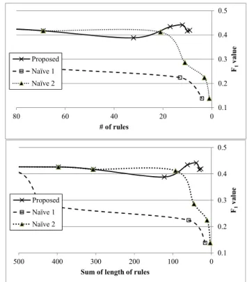
(7) 0.5. 0.8 0.7. 0.5. Naïve 1. 0.4. Naïve 2. Proposed. 0.3. Naïve 1 Naïve 2. F1 value. Proposed. 0.4. F1 value. 0.6. 0.2. 0.3 0.2 150. 100. 50. 0. 0.1 80. 60. # of rules. 40 # of rules. 20. 0. 0.5. Proposed. 0.3. Naïve 1 Naïve 2. F1 value. 0.4. 0.2 0.1. 500. Figure 2. Overview of the experiment result (Mylyn). F.. Comparison with Other Methods. We compare the proposed with other rule reduction methods, namely “naïve 1” and “naïve 2.” The naïve 1 method is a conventional rule reduction method that relies on the threshold in confidence only. Rules can be reduced by increasing the threshold confidence. The naïve 2 method is a combination of the naïve 1 method and a rule removal method that eliminates long rules subsumed by shorter rules. This method is intended to understand how much rules are subsumed by other rules. In this method, the shortest rules are selected based on a given threshold confidence; then, longer rules are selected unless they are not subsumed by shorter rules. Also, we compare with four commonly used machine learning techniques: logistic regression, random forest, CART and naïve Bayes classifier.. G.. Experimental Procedure. Given an initial rule set of Mylyn (Table IV), we run the proposed algorithm (Fig.1) with different threshold values, from improvement = 0 up to 0.15 where all “length ≥ 3” rules were removed. For each reduced rule set, we apply it to the Mylyn v2.0 dataset and compute evaluation criteria shown in Section IV.E. Similarly, for Eclipse PDE rule set, we run the proposed algorithm with improvement = 0 up to 0.3; and, for each reduced rule set, we apply it to the Eclipse PDE v3.2 dataset for performance evaluation. We run naïve 1 and 2 methods, which removes rules whose confidence values are smaller than the given threshold confidence.. 400. 300 200 Sum of length of rules. 100. 0. Figure 3. Overview of the experiment result (Eclipse PDE) For Mylyn dataset, we start with confidence = 0.78 up to 0.95 where all “length ≤ 3” rules were removed. Similarly, for Eclipse PDE dataset, we start with confidence = 0.70 up to 0.86.. V. RESULT AND DISCUSSION A.. Result 1: Comparison with Naïve Rule Reduction Methods. Fig.2 and 3 show the overview of the result for Mylyn and Eclipse PDE respectively. The upper graph shows reduction of the number of rules, and the lower graph shows the reduction of the total rule length. As the number of rules and the total rule length reduces, the conventional method (naïve 1), which reduces rules by the threshold in confidence, loses prediction accuracy (in terms of F1 value.) On the contrary, our proposed method sustains high prediction accuracy. Regarding the naïve 2 method, it showed better performance than the naïve 1 method, which indicates the effectiveness of eliminating long rules that are subsumed by shorter rules. In Mylyn dataset, 1287 out of 1347 (95.5%) rules were subsumed by shorter rules. However, giving higher threshold confidence and the number of rules became smaller than 60, the prediction accuracy dropped down much more than the proposed method. This indicates the proposed method’s advantage of setting thresholds based on the length of rules. Similarly in Eclipse PDE dataset, the naïve 2 method did better than the naïve 2 method; however, when the number of rules became smaller than 20, the prediction accuracy dropped down greatly..
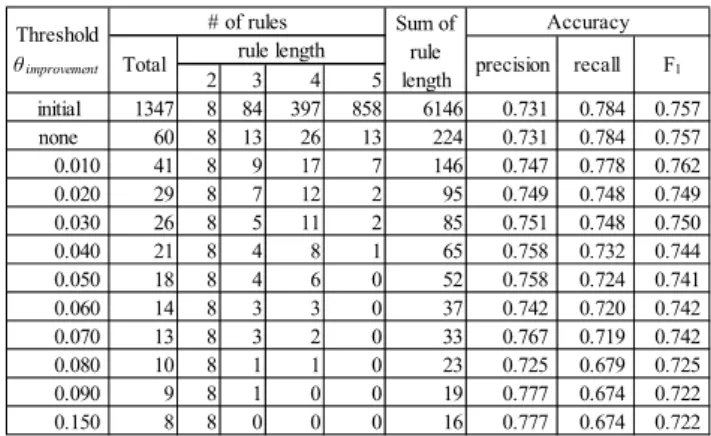
(8) Table VI (a). Rule reduction by the proposed method (Mylyn) Threshold θ improvement initial none 0.010 0.020 0.030 0.040 0.050 0.060 0.070 0.080 0.090 0.150. Total 1347 60 41 29 26 21 18 14 13 10 9 8. # of rules rule length 2 3 4 8 84 397 8 13 26 8 9 17 8 7 12 8 5 11 8 4 8 8 4 6 8 3 3 8 3 2 8 1 1 8 1 0 8 0 0. 5 858 13 7 2 2 1 0 0 0 0 0 0. Accuracy Sum of rule precision recall length 6146 0.731 0.784 224 0.731 0.784 146 0.747 0.778 95 0.749 0.748 85 0.751 0.748 65 0.758 0.732 52 0.758 0.724 37 0.742 0.720 33 0.767 0.719 23 0.725 0.679 19 0.777 0.674 16 0.777 0.674. F1 0.757 0.757 0.762 0.749 0.750 0.744 0.741 0.742 0.742 0.725 0.722 0.722. Table VI (b). Rule reduction by the naïve 1 method (Mylyn) Threshold θ confidence initial 0.78 0.80 0.85 0.88 0.90 0.92 0.93 0.94 0.95 1.00. Total 1347 999 841 397 184 106 64 44 38 30 23. # of rules rule length 2 3 4 8 84 397 6 59 289 3 51 247 1 15 105 0 6 44 0 2 27 0 2 14 0 1 9 0 1 8 0 0 6 0 0 5. 5 858 645 540 276 134 77 48 34 29 24 18. Accuracy Sum of rule precision recall length 6146 0.731 0.784 4570 0.757 0.760 3847 0.756 0.733 1847 0.790 0.614 864 0.827 0.520 499 0.856 0.449 302 0.848 0.312 209 0.842 0.256 180 0.843 0.235 144 0.879 0.175 110 0.867 0.098. F1 0.757 0.758 0.744 0.691 0.639 0.590 0.456 0.393 0.368 0.292 0.176. Table VI (c). Rule reduction by the naïve 2 method (Mylyn) Threshold θ confidence initial none 0.78 0.80 0.85 0.88 0.90 0.92 0.93 0.94 0.95. Total 1347 60 48 59 50 38 26 19 13 11 7. # of rules rule length 2 3 4 8 84 397 8 13 26 6 8 25 3 18 26 1 4 29 0 6 15 0 3 15 0 2 5 0 1 6 0 1 6 0 0 6. 5 858 13 9 12 16 17 8 12 6 4 1. Accuracy Sum of rule precision recall length 6146 0.731 0.784 224 0.731 0.784 181 0.757 0.760 224 0.756 0.733 210 0.790 0.614 163 0.827 0.520 109 0.856 0.449 86 0.848 0.312 57 0.842 0.256 47 0.843 0.235 29 0.879 0.175. F1 0.757 0.757 0.758 0.744 0.691 0.639 0.590 0.456 0.393 0.368 0.292. Details of results are shown in Table VI and VII. For Mylyn dataset, in Table VI (a), the proposed method could reduce the number of rules from 1347 down to 13, while the delta of the prediction performance is only .015 (from .757 down to .742) in terms of the F1 value. On the other hand, in Table VI (b) and (c), naïve 1 and 2 methods could also reduce the number of rules, however, F1 value became extremely low. For example, when the number of rules is reduced down to 23 in the naïve 1 method, F1 value became .176, which is very low (Table VI(b).) Also in naïve 2 method, when the number of rules is reduced down to 19, F1. Table VII (a). Rule reduction by the proposed method (Eclipse PDE) Threshold θ improvement initial none 0.020 0.050 0.070 0.100 0.200 0.300. Total 398 89 69 32 17 12 10 9. # of rules rule length 2 3 4 0 9 80 0 9 30 0 9 21 0 9 20 0 9 5 0 9 3 0 9 1 0 9 0. 5 309 50 39 3 3 0 0 0. Accuracy Sum of rule precision recall length 1892 0.336 0.582 397 0.336 0.582 306 0.333 0.557 122 0.362 0.417 62 0.508 0.380 39 0.583 0.354 31 0.565 0.329 27 0.578 0.329. F1 0.426 0.426 0.417 0.388 0.434 0.441 0.416 0.419. Table VII (b). Rule reduction by the naïve 1 method (Eclipse PDE) Threshold θ confidence initial 0.70 0.75 0.76 0.83 0.84 0.86. Total 398 330 108 92 92 13 4. # of rules rule length 2 3 4 0 9 80 0 8 67 0 2 19 0 2 17 0 2 17 0 1 4 0 1 2. 5 309 255 87 73 73 8 1. Accuracy Sum of rule precision recall length 1892 0.336 0.582 1567 0.333 0.557 517 0.519 0.341 439 0.485 0.203 439 0.485 0.203 59 0.579 0.139 16 0.750 0.076. F1 0.426 0.417 0.412 0.286 0.286 0.224 0.138. Table VII (c). Rule reduction by the naïve 2 method (Eclipse PDE) Threshold θ confidence initial none 0.70 0.75 0.76 0.83 0.84 0.86. Total 398 89 69 21 11 11 3 1. # of rules rule length 2 3 4 0 9 80 0 9 30 0 8 22 0 2 8 0 2 6 0 2 6 0 1 2 0 1 0. 5 309 50 39 11 3 3 0 0. Accuracy Sum of rule precision recall length 1892 0.336 0.582 397 0.336 0.582 307 0.333 0.557 93 0.519 0.341 45 0.485 0.203 45 0.485 0.203 11 0.579 0.139 3 0.750 0.076. F1 0.426 0.426 0.417 0.412 0.286 0.286 0.224 0.138. value became .456 (Table VI (c).) Similarly in Eclipse PDE dataset, the proposed method outperformed both naïve 1 and 2 methods. The proposed method was able to reduce the number of rules from 398 down to 12, while the prediction performance even improved from .426 to .441 (Table VII (a).) Regarding the ease of understanding of a rule set, the proposed method could effectively reduce the complex (long) rules. In Table VII (a), when the number of rules is 13, all longest (length = 5) rules were removed. On the other hand, in naïve 1 and 2 methods, the longest rules were always remaining. Also, shortest (length = 2) rules disappeared as the rule set reduced in the naïve methods. Similar result exhibits in the experiment based on Eclipse PDE..
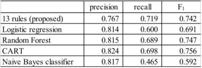
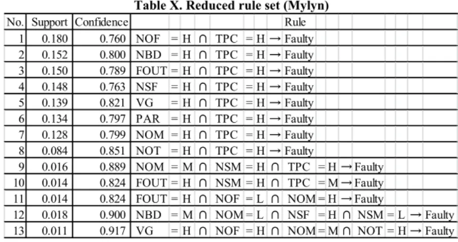
(9) Table VIII. Comparison with commonly used machine learners (Mylyn). 13 rules (proposed) Logistic regression Random Forest CART Naive Bayes classifier. precision 0.767 0.814 0.815 0.824 0.817. recall 0.719 0.600 0.689 0.698 0.465. F1 0.742 0.691 0.747 0.756 0.592. Table IX. Comparison with commonly used machine learners (Eclipse PDE). 12 rules (proposed) Logistic regression Random Forest CART Naive Bayes classifier. B.. precision 0.583 0.889 0.625 0.330 0.567. recall 0.354 0.101 0.253 0.456 0.215. F1 0.441 0.182 0.360 0.383 0.312. Result 2: Comparison with Commonly Used Machine Learners. Table VIII and XI show the prediction performance of commonly used machine learners, compared with the proposed method (i.e. prediction by the reduced rule set) in Mylyn and Eclipse PDE respectively. In Mylyn dataset (Table VIII), the proposed method and tree-based methods (Random Forest and CART) outperformed other two methods (logistic regression and naïve Bayes classifier) in terms of F1 value. In Eclipse PDE dataset (Table IX), the proposed method outperformed other four methods in F1 value. These results indicate that the proposed association rule mining approach is able to produce accuracy that is comparative to commonly used machine learners.. C.. Discussion. Table X shows the details of rules in the reduced rule set (13 rules) derived by the proposed method with a threshold improvement = .07 in Mylyn dataset. Although interpretation of rules itself is not the main scope of this paper, here we try to give a possible interpretation of rules. (Due to page limitation, this Section investigates Mylyn dataset only.) There are 8 shortest (length=2) rules, and all of them consist in their antecedent “TPC = H,” which means the number of revisions of a file is high (TPC ≥ 3.) This indicates the frequent revisions to a module is the most influential factor of fault injection in the Mylyn dataset. This corroborates the results of previous studies [2][15][17]. However, the condition “TPC = H” alone is not sufficient to have a consequent “faulty.” Looking at rules no. 1-8 in Table X, either of “NOF = H”, “NBD = H”, “FOUT = H”, “NSF = H”, “VG = H”, “PAR = H”, “NOM = H” or “NOT = H” is needed in addition to “TPC = H” to have a fault with high confidence level (≥ 0.75.) These metrics include control flow complexity (NBD and VG), data complexity (PAR, NOF and NSF), inter-module complexity (FOUT) and size metrics (NOM and NOT). Therefore, it can be interpreted as that the fault is injected when the revision to a module is frequent and the module has high complexity or its size is large.. Next we focus on rules no.9 and no.10. It can be considered that these rules expand the preconditions of shorter rules no.7 and no.3. While the rule no.7 requires NOM to be “H”, the rule no.9 allows “NOM = M” by adding “NSM = H” to its antecedent. Similarly, while the rule no.3 requires TPC to be “H”, the rule no.10 allows “TPC = M” by adding “NSM = H.” Next we focus on the rule no.11. Interestingly, this rule consists in its antecedent “NOF = L”, which means the number of attributes = zero. At the same time, this rule requires “FOUT = H” (the number of method calls of a file ≥33) and “NOM = H” (the number of methods ≥8). These characterize a module having no attributes while it has many methods and many method calls to other classes. On the other hand, the rule no.12 consists “NOM = L” (the number of methods ≤ 2), “NBD = M” (nested block depth = 1), “NSF = H” (the number of static attributes ≥ 1) and “NSM = L” (the number of static methods = 0). This indicates that a module of less branching complexity with just one or two methods can have a fault if it has one or more static attributes. Finally, the rule no.13 consists of many complexity metrics included in the shortest rules, while it does not consist TPC, which is the most influential factor of fault injection. This indicates that regardless of the frequency of revisions, a module can have a fault if the module is complex enough. The analysis above confirmed that interpretation of a rule set became possible by our proposed rule reduction algorithm.. D.. Threats to Validity. In this section, we discuss the threats to the validity of our work. We used datasets collected from two projects. We need to analyze other open source and closed source systems to generalize our results. In addition, the set of metrics used to extract association rules is by no means complete. Thus, using other metrics may yield different results. However, we believe that the same approach can be applied on any set of metrics. We used recall, precision and F1-value to evaluate the prediction performance of rule sets. We need to use other criteria such as ROC curves [10] to increase the reliability of our results. This study obtains the number of faults in source code files using the SZZ algorithm. The algorithm is commonly used in fault prediction researches [13][15], but has the limitation that faults not recorded in CVS log comments cannot be collected. Further research is required to improve the accuracy of faults collection from repositories. To mine enough initial rules before applying our rule reduction method, this paper set threshold values support = .01 and confidence = .75 for Mylyn v.1.0 dataset and support = .02 and confidence = .65 for Eclipse PDE v3.1 dataset. Since these values may affect the result of rule reduction and prediction, we need to conduct further experiments using different values. We used rules whose consequent is “faulty” only, where nonfaulty rules are ignored. Although we could obtain promising prediction accuracy with faulty rules only, further research is required to confirm whether non-faulty rules are indeed needless or not in fault prediction. To use both faulty and non-faulty rules, one of the issues we need to address in future is how to conduct prediction for modules that are not included in both faulty and non-faulty rules..
(10) Table X. Reduced rule set (Mylyn) No. Support Confidence Rule 1 0.180 0.760 NOF = H ∩ TPC = H → Faulty 2 0.152 0.800 NBD = H ∩ TPC = H → Faulty 3 0.150 0.789 FOUT = H ∩ TPC = H → Faulty 4 0.148 0.763 NSF = H ∩ TPC = H → Faulty 5 0.139 0.821 VG = H ∩ TPC = H → Faulty 6 0.134 0.797 PAR = H ∩ TPC = H → Faulty 7 0.128 0.799 NOM = H ∩ TPC = H → Faulty 8 0.084 0.851 NOT = H ∩ TPC = H → Faulty 9 0.016 0.889 NOM = M ∩ NSM = H ∩ TPC = H → Faulty 10 0.014 0.824 FOUT = H ∩ NSM = H ∩ TPC = M → Faulty 11 0.014 0.824 FOUT = H ∩ NOF = L ∩ NOM = H → Faulty 12 0.018 0.900 NBD = M ∩ NOM = L ∩ NSF = H ∩ NSM = L → Faulty 13 0.011 0.917 VG = H ∩ NOF = H ∩ NOM = M ∩ NOT = H → Faulty. VI. CONCLUSION To reveal the insights and better understanding of the causes of faulty modules, this paper proposed a novel technique to reduce association rules that can eliminate long and/or similar rules yet sustaining the desirable prediction performance as much as possible. Our major findings based on an empirical evaluation with the Mylyn dataset and the Eclipse PDE dataset include the following: . In the Mylyn dataset, the proposed method reduces the number of rules from1347 down to 13, while the delta of the prediction performance was only .015 (from .757 down to .742) in terms of the F1 value. And, in the Eclipse PDE dataset, the proposed method reduces the number of rules from 398 to 12, while the prediction performance even improved (from .426 to .441.). . On the other hand, two naïve rule reduction methods, which simply remove rules whose confidence values are smaller than the given threshold, could also reduce the number of rules, but in these cases the prediction performance became extremely low.. . We compared our rule-based prediction with conventional model-based approaches such as logistic regression, random forest, CART and naïve Bayes classifier. As a result, the proposed association rule mining approach was able to produce accuracy that is comparative to commonly used machine learners. This indicates the reduced rule set is worthwhile and important.. . Through an analysis of a reduced rule set, it is confirmed that our proposed rule reduction technique provides a better understanding of the causes of faulty modules.. E. ACKNOWLEDGMENTS Part of this work was conducted under Japan Society for the Promotion of Science, Grant-in-Aid for Scientific Research (C) (22500028) and Young Scientists (A) (24680003).. F. REFERENCES [1] Agrawal, R., Imielinski, T. and Swami, A.: Mining Association Rules between Sets of Items in Large Databases, Proc. of 1993 ACM SIGMOD Int’l Conf. on Management of Data,Washington, D.C., USA, pp.207-216 (1993). [2] D'Ambros, M., Lanza, M., Robbes, R.: Evaluating Defect Prediction Approaches: a Benchmark and an Extensive. Comparison, Empirical Software Engineering, Published online, DOI 10.1007/s10664-011-9173-9, (2011). [3] Eclipse Mylyn Open Source Project, http://www.eclipse.org/mylyn/ [4] Eclipse Plug-in Development Environment (PDE), http://www.eclipse.org/pde/ [5] Hamano, Y., Amasaki, S., Mizuno, O. and Kikuno, T.: Application of Association rule mining to Analysis of Risk Factors in Software Development Projects, JSSST Computer Software, Vol.24, No.2, pp.79-87(2007). [6] Kamei, Y., Monden, A., and Matsumoto, K.: Empirical Evaluation of SVM-based Software Reliability Model, In Proc. 5th ACM-IEEE Int’l Symposium on Empirical Software Engineering (ISESE2006), Vol.2, pp.39-41(2006). [7] Kamei, Y., Monden, A., Morisaki, S., and Matsumoto, K.: A Hybrid Faulty Module Prediction Using Association Rule Mining and Logistic Regression Analysis, In Proc. 2nd Int’l Symposium on Empirical Software Engineering and Measurement (ESEM2008), pp.279-281(2008). [8] Kim, S., Whitehead, Jr., E. J., and Zhang, Y.: Classifying Software Changes: Clean or Buggy?, IEEE Trans. Softw. Eng., Vol.34, No.2, pp.181-196(2008). [9] Khoshgoftaar, T. M. and Allen, E. B.: Modeling Software Quality with Classification Trees, Recent Advances in Reliability and Quality Engineering, Singapore, World Scientific, pp.247-270(1999). [10] Lessmann, S., Baesens, B., Mues, C., Pietsch, S.: Benchmarking classification models for software defect prediction: A proposed framework and novel findings, IEEE Trans. on Software Engineering, vol.34, no.4, pp.485496(2008). [11] Li, P. L., Herbsleb, J., Shaw, M. and Robinson, B.: Experiences and Results from Initiating Field Defect Prediction and Product Test Prioritization Efforts at ABB Inc., Proc. 28th Int’l Conf. on Software Engineering, Shanghai,China, pp.413-422(2006). [12] Michail, A.: Data Mining Library Reuse Patterns Using Generalized Association Rules, Proc. 22nd International Conference on Software Engineering (ICSE’00), pp.167176(2000)..
(11) [13] Mizuno, O. and Kikuno, T., “Prediction of fault-prone software modules using a generic text discriminator,” IEICE Transactions on Information and Systems, vol. E91-D, no. 4, pp. 888–896, 2008. [14] Morisaki, S., Monden, A., Matsumura, T., Tamada, H., and Matsumoto, K.: Defect Data Analysis Based on Extended Association Rule Mining, Proc. 4th Int’l Workshop on Mining Software Repositories (MSR 2007), pp.17-24(2007). [15] Moser, R., Pedrycz, W., and Succi, G.: A comparative analysis of the efficiency of change metrics and static code attributes for defect prediction,” Proc. 30th International Conference on Software engineering (ICSE’08), pp. 181-190 (2008). [16] Munson, J. C. and Khoshgoftaar, T. M.: The Detection of Fault-prone Programs, IEEE Trans. Softw. Eng., Vol.18, No.5, pp.423-433(1992). [17] Nagappan, N., Ball, T.: Use of relative code churn measures to predict system defect density, In Proc. 27th Int’l Conf. on Software Engineering (ICSE2005), pp.284-292(2005). [18] Ohlsson, N. and Alberg, H.: Predicting Fault-Prone Software Modules in Telephone Switches, IEEE Trans. Softw. Eng., Vol.22, No.12, pp.886-894(1996). [19] She R., Chen F., Wang K., Ester M., Gardy J.L., Brinkman F.L.: Frequent-Subsequence-Based Prediction of Outer Membrane Proteins, Proceedings of 9th ACM SIGKDD. International conference on Knowledge Discovery and Data Mining, pp. 436-445, (2003). [20] Shihab, E., Mockus, A., Kamei, Y., Adams, B., Hassan, A. E.: High-Impact Defects: A Study of Breakage and Surprise Defects, Proc. ACM SIGSOFT Symposium on the Foundations of Software Engineering (FSE2011), pp.300310(2011). [21] Shihab, E., Jiang, Z. M., Ibrahim, W. M., Adams, B. and Hassan, A. E.: Understanding the Impact of Code and Process Metrics on Post-release Defects: A Case Study on the Eclipse Project, Proc. 2010 ACM-IEEE International Symposium on Empirical Software Engineering and Measurement (ESEM2010), pp.1-10(2010). [22] Song, Q., Shepperd, M., Cartwright, M. and Mair, C.: Software Defect Association Mining and Defect Correction Effort Prediction, IEEE Trans. Softw. Eng., Vol.32, No.2, pp. 69-82(2006). [23] Śliwerski, J, Zimmermann, T., and Zeller, A.: When do changes induce fixes? Proc. Int’l Conference on Mining Software Repositories (MSR’05), pp.1-5(2005). [24] Understand, Scientific http://www.scitools.com/. Toolworks,. Inc.,. [25] Yang, Q., Zhangand, H.H. and Li, T.: Mining Web Logs for Prediction Models in WWW Caching and Prefetching, Proc. of 7th ACM SIGKDD Int’l Conf. of Knowledge Discovery and Data Mining, California , USA, pp. 473-478 (2001)..
(12)
図
+3
関連したドキュメント