An approximation scheme for optimal stochastic control problems (Financial Modeling and Analysis)

(1)

An

approximation

scheme for optimal

stochastic control

problems*

Yumiharu Nakano

Graduate School ofInnovation Management

Tokyo Institute ofTechnology

1 Introduction

Weconsider the optimal stochastic controlproblemsover afinite horizon $T\in(0, \infty)$ withvalue

function

$v(t, x)= \inf_{\alpha\in}E[f(X_{T}^{t,x,\alpha})+l^{T}g(s, X_{s}^{t,x,\alpha}, \alpha_{s})ds], (t, x)\in[O, T]\cross \mathbb{R}^{m}$, (1.1)

where the controlled process $\{X_{s}^{t,x,\alpha}\}$ is governedby

$[Matrix]$

(1.2)

Here, $\mu$: $[0, T]\cross \mathbb{R}^{m}\cross Aarrow \mathbb{R}^{m},$$\sigma$ : $[0,T]\cross \mathbb{R}^{m}\cross Aarrow \mathbb{R}^{m\cross d},$ $f$ :$\mathbb{R}^{m}arrow \mathbb{R},$ $g$ : $[0, T]\cross \mathbb{R}^{m}\cross Aarrow \mathbb{R}$

and $A\subset \mathbb{R}^{k}$

.

The conditions imposed

on

these functions

are

described in

Section

2

below.

The

process $\{W_{s}\}_{0\leq t\leq T}$is

a

$d$-dimensional standardBrownian motionon a filteredprobability space

$(\Omega, \mathcal{F}, \{\mathcal{F}_{t}\}_{0\leq t\leq T}, \mathbb{P})$ satisfying the usual conditions. The class

$\mathcal{A}$ofcontrols isthecollection of

$A$-valued $\{\mathcal{F}_{t}\}_{0\leq t\leq T}$-progressively measurable processes $\{\alpha_{t}\}_{0\leq t\leq}\tau.$

One ofthemainapproachesforoptimalstochastic controlproblemsistosolve the

Hamilton-Jacobi-Bellman (HJB) equation that the value function should satisfy, and then to construct

a

control strategy via the verification argument. For

our

problem (1.1), the corresponding HJB

equation is given by

$-\partial_{t}v+F(t, x, Dv, D^{2}v)=0, (t, x)\in[O, T)\cross \mathbb{R}^{m}$, (1.3)

with the terminal condition$v(T, x)=f(x),$ $x\in \mathbb{R}^{m}$, where

$F(t, x,p, M)= \sup_{a\in A}\{-\mu^{*}(t, x, a)p-\frac{1}{2}tr((\sigma\sigma^{*})(t,x, a)M)-g(t, x, a)\}$

for $x\in \mathbb{R}^{m},$ $p\in \mathbb{R}^{m}$, and $M$, a symmetric and nonnegative definite $m\cross m$ matrix. Here we

have denoted by $\partial_{t}$ the partial differential operator with respect to the time variable

$t$, by $D^{j}$

the j-th order partial differential operator with respect to the space variable$x$, and by $c^{*}$ the

transposeof amatrix $c.$

Since analytical solutions for HJB equations

are

rarely available,

a

number of numerical

methods have been proposed in the literature. However, for practical applications there still

remain several challenging problems. First one is that in

some

schemes the coefficients of the

(2)

finite-difference scheme (see, e.g., Kushner and Dupuis [13]), the diffusion matrix $\sigma\sigma^{*}$ in

our

notation should basically be diagonally dominant. Althoughthisrestriction

can

beweakenedby

considering thegeneralized

finite-difference

that involves a nontrivial adjustmentofthe diffusion

matrix,

we

may need

a

large size ofthe stencil depending

on

a problem, as well

as

thefurther

computational efforts for the implementation. See Bonnans and Zidani [3], Bonnans et al. [2]

andthe references therein. The optimal quantization approachtaken by Pag\‘es et al. [17] works

under mildconditionson the coefficients, in particular, under quadratic growthconditions on $f$

and $g$

.

However, their scheme requires most components of the process $\{X_{s}^{x,\pi}\}$ being actually

control-free. InFahimet al. [8], theyextract

an

uncontrolled generator from the nonlinearity$F,$

and then

use

aprobabilistic representationof the HJB equationbasedon the process associated

with such generator. Then the partial derivatives of the value functionin that representation

are computedby theexpectations of random variables involving the valuefunctionitself via the

integration-by-parts. These tricks cost

some

strong non-degeneracy conditions

on

$F.$

Secondproblemiscomputationaldifficulties in high-dimensional

cases.

In general, the

finite-difference scheme needs a spatial grid with its size growing exponentially as the dimension $m$

becomeslarge. As forthe method by [17], the quantization

error

with respectto

an

$\ell$-dimensional

randomvariableisknownto be$O(N^{1/\ell})$ ifwe denoteby $N$the number of discretizing pointsfor

the random variable. The scheme by [8] can be applied to high-dimensional problems because

it is

based

on Monte Carlosimulationforcomputing theconditionalexpectation, butthekernel

density estimationused in this procedure is in general suffered from thecurse-of-dimensionality.

The finite-element like schemes studied by e.g., Camilli and Falcone [5] and Debrabant and

Jakobsen [7], often called Semi-Lagrangian schemes, solve the first problem. That is, their

scheme converge to the original value functions under no special assumption on the diffusion

matrix $\sigma\sigma^{*}$. The difficulty in their scheme

is that they require the interpolation of the value

functions

in the state space, and need involvedcomputational proceduresfor theimplementation

in high-dimensional problems (see Carlini et al. [6]).

In thispaper, we propose a new time-discretization schemefor the problem (1.1). Itis based

on a

probabilistic representation for the convolution of$v$ by

a

probability density function. In

Section 2 below, we first give a rough derivation ofthe semi-discrete scheme, and then prove

its convergence results by the viscosity solution method presented in Barles and Souganidis

[1]. With the choices of the kernel and with the estimation methods for the conditional

expec-tations, various numerical methods can be generated. Resulting numerical methods allow us

to

use

uncontrolled Markov processes to estimate the conditional expectations in the dynamic

programmingprocedure. Moreover, they can be implemented without the interpolation of the

value function or the adjustment of the diffusion matrix. We present one of possible methods

with

Gaussian distributions

in

Section 3.

$A$ numerical experiment is also performed there. We

focus on an artificialproblemhaving two-dimensional state space, where an analytical solution

for (1.3) is easilyobtained.

Throughout this paper, wewrite $|a|=( \sum_{i,j}a_{i,j}^{2})^{1/2}$ for amatrix $a=(a_{i,j})$

.

By$C$ we denote

(3)

2 Approximation of the value function

We discuss the general stochastic controlproblem (1.1) under the following assumptions onthe

coefficients:

Assumption 2.1 1. The

_functions

$\mu,$$\sigma,$$f,g$

are

Borel measumble withrespectto $(t, x, a)$ and

continuous with respect to $(t, x)$ uniformly

over

$a.$

2. There exists

a

positive constant $K$ such that,

for

every $s,$$t\in[0, T],$ $x,$$y\in \mathbb{R}^{m}$ and$a\in A,$

$|\mu(t,x, a)|+|\sigma(t,x, a)|\leq K(1+|x|)$,

$|\mu(s, x, a)-\mu(t, y, a)|+|\sigma(s,x, a)-\sigma(t, y, a)|\leq K|s-t|+K|x-y|,$ $|f(x)|+|g(t, x, a)|\leq K.$

With these conditions, the controlled stochastic differential equation (1.2) has aunique strong

solution for each control $\alpha\in \mathcal{A}$ (see, e.g., Fleming and

Soner

[9]

or

Krylov [12]) and the value

function$v$in(1.1)becomes

bounded.

Moreover, it is known that$v$satisfies the viscosity solution

property. To be precise, recallthat

an

$\mathbb{R}$-valued, upper-semicontinuous function$u$

on

$[0, T]\cross \mathbb{R}^{m}$

issaidto be

a

viscositysubsolution of(1.3) if,for any$(t,x)\in[O, T)\cross \mathbb{R}^{m}$and any smooth function

$\varphi$ such that $u-\varphi$has a local maximum at $(t, x)$ we have

$-\partial_{t}\varphi(t, x)+F(t, x, D\varphi(t, x), D^{2}\varphi(t, x))\leq 0.$

Similarly, an $\mathbb{R}$-valued, lower-semicontinuous function$u$ on $[0, T]\cross \mathbb{R}^{m}$ is said to be

a

viscosity supersolution of(1.3) if, forany $(t, x)\in[0, T)\cross \mathbb{R}^{m}$ andanysmoothfunction $\varphi$such that$u-\varphi$

has

a

local minimum at $(t, x)$ we have

$-\partial_{t}\varphi(t, x)+F(t, x, D\varphi(t, x), D^{2}\varphi(t,x))\geq 0.$

Wesay that$u$ isa viscosity solution of(1.3) ifit is both a viscosity subsolution and

a

viscosity

supersolution of (1.3). Then, Theorem 4.3.1 in Pham [19] tells

us

that

our

value function $v$

is indeed

a

viscosity solution of (1.3). In addition, by Theorem

4.4.5

in [19] the following

comparison principle holds: foreverybounded, upper-semicontinuous viscosity subsolution$u$of

(1.3) and bounded lower-semicontinuous viscosity supersolution $w$ of(1.3) such that $u(T, x)\leq$

$w(T, x),$ $x\in \mathbb{R}^{m}$,

we

have

$u(t, x)\leq w(t,x) , (t, x)\in[0, T]\cross \mathbb{R}^{m}.$

Let $\{t_{i}\}_{i=0}^{n}$ be a fixed set of time indices such that $0=t_{0}<t_{1}<\cdots<t_{n}=T$ with

$h=t_{i}-t_{i-1}=T/n,$ $i=1,$$\ldots,$$n$

.

We consider $n$ sufficiently large

so

that $h\in(0,1]$

.

To find

a

time discretization scheme for the valuefunction, first wewrite down the dynamic programming

principle

as

follows:

(4)

Replacing by its Euler-Maruyama approximation$\hat{X}_{t_{i+1}}^{t_{i},x,a}$ defined by

$\hat{X}_{s}^{t,x,a}=x+\mu(t, x, a)(s-t)+\sigma(t, x, a)\sqrt{s-t}G, t\leq s\leqt+h, a\in A,$

formally

we

have

$\mathbb{E}[v(t_{i+1}, X_{t_{i+}}^{t_{i},x}i^{\alpha})+\int_{t_{i}}^{t_{i+1}}g(s, X_{s^{i}}^{t,x,\alpha}, \alpha_{s})ds]\approx \mathbb{E}[v(t_{i+1},\hat{X}_{t_{i+1}}^{t_{i},x,\alpha_{t_{i}}})]+hg(t_{i}, x, \alpha_{t_{i}})$.

Here, $G=(G_{1}, \ldots, G_{d})^{*}$is arandom variable such that $G_{i}$’s

are

mutually independent and that

$\mathbb{E}[G_{i}]=0, E[G_{i}G_{j}]=\delta_{ij}, \mathbb{E}[|G_{i}|^{3}]<\infty,i,j=1, \ldots, d$, (2.1)

where $\delta_{ij}$ denote the Kronecker’s delta.

Now

we

consider the convolution $\phi^{h}*v(t_{i+1}, \cdot)$ by

some

kernel $\phi^{h}$ to approximate $v(t_{i+1}, \cdot)$

.

To this end, let $\phi$ be a probabilitydensity function on $\mathbb{R}^{m}$ with full support, i.e., _$\phi(y)>0$ for

all $y\in \mathbb{R}^{m}$, andthen define

$\phi^{h}(x):=\frac{\phi(x/\lambda(h))}{\lambda(h)^{m}}, x\in \mathbb{R}^{m},$

where$\lambda$isapositivefunction on

$(0,1]$. Then,for any bounded function$u$, the convolution $\phi^{h}*u$

can berepresented as

$( \phi^{h}*u)(x+\xi)=\int_{\mathbb{R}^{m}}u(z)\frac{\phi((x+\xi-z)/\lambda(h))}{\lambda(h)^{m}}dz$

$= \int_{\mathbb{R}^{m}}u(x+\lambda(h)z)\phi(\frac{\xi}{\lambda(h)}-z)dz, x, \xi\in \mathbb{R}^{m}.$

Let $\mathcal{D}^{h}$

be a subset of$\mathbb{R}^{m}$ satisfying

$\int_{\mathbb{R}^{m}\backslash \mathcal{D}^{h}}\phi(\xi/\lambda(h)-z)dzarrow 0,$ $h\searrow 0$, and let $\psi^{h}$ be an

another probability density function having $\mathcal{D}^{h}$

as

the support set. Then, roughly speaking,

$(\phi^{h}*u)(x+\xi)$ is _approximated_by _{$\int_{\mathcal{D}^{h}}u(x+\lambda(h)z)\phi(\xi/\lambda(h)-z)dz$}_and _this

_can

_be_written

_as

$\int_{\mathcal{D}^{h}}u(x+\lambda(h)z)\phi(\frac{\xi}{\lambda(h)}-z)dz=\int_{\mathcal{D}^{h}}u(x+\lambda(h)z)\phi(\frac{\xi}{\lambda(h)}-z)\frac{\psi^{h}(z)}{\psi^{h}(z)}dz$

$= \mathbb{E}[u(x+\lambda(h)Z^{h})\phi(\frac{\xi}{\lambda(h)}-Z^{h})\frac{1}{\psi^{h}(Z^{h})}],$

where$Z^{h}$ isarandom variable with probability density$\psi^{h}$, which is assumed to be independent

of$G$

.

Thus, denoting $H_{h}^{t,x,a}=\mu(t, x, a)h+\sigma(t, x, a)\sqrt{h}G$, we_have

$\mathbb{E}[(\phi^{h}*u)(\hat{X}_{t+h}^{t,x,a})]\approx \mathbb{E}[\mathbb{E}[u(x+\lambda(h)Z^{h})\phi(\frac{H_{h}^{t,x,a}}{\lambda(h)}-Z^{h})\frac{1}{\psi^{h}(Z^{h})}|H_{h}^{t,x,a}]]$

$= \mathbb{E}[u(x+\lambda(h)Z^{h})\phi(\frac{H_{h}^{t,x,a}}{\lambda(h)}-Z^{h})\frac{1}{\psi^{h}(Z^{h})}].$

The last expression mightbe useful since theargument of$u$ is control-free. Then,

as

$\lambda(h)\searrow 0,$

the quantity $\mathbb{E}[(\phi^{h}*u)(\hat{x}_{t}^{t}\dotplus_{h}^{x,a})]$ converges to $\mathbb{E}[u(\hat{x}_{t}^{t}\dotplus^{x_{h}a})]$ under mild conditions on

$u$, so we

expect that the schemedefined by

(5)

with

$\Phi^{h}[u](t, x)=\inf_{a\in A}\{E[u(x+\lambda(h)Z^{h})\phi(\frac{H_{h}^{t,x,a}}{\lambda(h)}-Z^{h})\frac{1}{\psi^{h}(Z^{h})}]+hg(t, x, a)\}$

gives

an

approximationforthe value function$v.$

Let $\beta$ be

a

function

on

$(0,1]$ defined by

$\beta(h)=\sup_{t\in l0,T|,\xi\in R^{m} ,a\in A}\mathbb{E}\int_{\mathbb{R}^{m}\backslash \mathcal{D}^{h}}\phi(\frac{H_{h}^{t,\xi,a}}{\lambda(h)}-z)dz$. (2.2)

Then

we are

able to statethe following convergence result.

Theorem 2.2 Let $v$ : $[0, T]\cross \mathbb{R}^{m}arrow \mathbb{R}$ be

defined

by (1.1). Suppose that Assumption

2.1

is

satisfied.

Suppose also that

$\lim_{h\searrow 0}\frac{\lambda(h)+\beta(h)}{h}=0.$

Then,

$v^{h}(t_{i}, y) arrow v(t, x)$

as

$h\searrow 0,$ $t_{i}arrow t$, and_{$yarrow x$}, uniformly

on

any compact subset

of

$\mathbb{R}^{m}.$

Toobtain the ratesof convergenceof

our

schemes,

we

impose

more

regularity conditions

on

the coefficients.

Assumption 2.3 There exist positive

constants

$K’$ such that,

for

every

$s,$$t\in[0, T],$ $x,$$y\in \mathbb{R}^{m}$

and $a\in A,$

$|f(x)-f(y)|+|g(s, x, a)-g(t, y, a)|\leq K’|x-y|+K’|s-t|^{1/2},$

$|\mu(t, x, a)|\leq K’, |\sigma(t, x, a)|\leq K’.$

Theorem 2.4 Let$v:[0, T]\cross \mathbb{R}^{m}arrow \mathbb{R}$ be

defined

by (1.1). Suppose that Assumptions

2.1

and

2.3 are

_satisfied.

Suppose also that $E[G_{i}^{3}]=0,$ $E[G_{i}^{4}]<\infty,$ $i=1,$

$\ldots,$

$d$

.

If

$\lambda$ and $\beta$ satisfy

$\lambda(h)+\beta(h)\leq Ch^{7/6}$, then we have

$0 \leq i\leq n\max|v^{h}(t_{i}, x)-v(t_{i}, x)|\leq Ch^{1/6}, x\in \mathbb{R}^{m}.$

Furthermore,

_if

$\lambda(h)+\beta(h)\leq Ch^{3/2}$ then

we

obtain

$-Ch^{1/6}\leq v(t_{i}, x)-v^{h}(t_{i}, x)\leq Ch^{1/4}, x\in \mathbb{R}^{m}, i=1, \ldots, n.$

3

$A$

fully

numerical method

Throughout this section, we suppose that Assumptions 2.1 and 2.3

are

satisfied. We take the

$\mathbb{R}^{d}$-valued random variable $G=G^{M,q}$

as an

optimally quantized random variable in the

sense

that $G^{M,q}$ isaminimizer of

(6)

randomvariables with -supporting points, where and isa -dimensional

standard

Gaussian

random variable. We refer to Grafand Luschgy [10] for

a

detailed account

of optimal quantization theory, and to Pag\’es and Printems [18] for numerical procedures for

obtaining $G^{M,2}$

.

Set

$G^{M,q}(\Omega)=\{\gamma_{1}, \ldots, \gamma_{M}\}, \mathbb{P}(G^{M,q}=\gamma_{i})=p_{i}, i=1, \ldots, M.$

In most of numerical realizations, the random variables$G^{M,q\prime}s$approximatelysatisfy the moment

condition (2.1). $A$reasonwhywe usethe quantization is thatweneedsufficientlymany_{points of}

$H_{h}^{t,x,a}/\lambda(h)$’s

near

its

mean

tobeshot by MonteCarlo simulations of Gaussianrandom variables,

with less number ofcomputations. See the comment made just after (3.2) below.

We choose thefunction $\lambda$

as

$\lambda(h)/harrow 0, h\searrow 0.$

For example, we maytake $\lambda(h)=h/(-\log h)$.

Todescribe the realizations of$H^{t,x,a}$

$h$ , weput

$\eta_{i}^{h}(t, x, a)=\mu(t, x, a)h+\sigma(t, x, a)\sqrt{h}\gamma_{i}, i=1, \ldots, M.$

As

the

functions

$\phi$ and $\psi^{h}$,

we

examine

$\phi(y)=\frac{e^{-|\xi|^{2}/2}}{(2\pi)^{m/2}}, \psi^{h}(y)=\frac{e^{-|\xi|^{2}/(2\tau(h))}}{(2\pi\tau(h))^{m/2}}, y\in \mathbb{R}^{m},$

where$\tau(h)>0.$

Let $Z$be an_$m$-dimensionalstandard Gaussian_{random variable. Then} $\Phi^{h}[u]$ isdescribed by

$\Phi^{h}[u](t, x)=\inf_{a\in A}\{\sum_{j=1}^{M}p_{j}\mathbb{E}[u(x+\lambda(h)\sqrt{\tau(h)}Z)\phi(\frac{\eta_{j}^{h}(t,x,a)}{\lambda(h)}-\sqrt{\tau(h)}Z)\frac{1}{\psi^{h}(\sqrt{\tau(h)}Z)}]$

$+hg(t, x, a)$ _.

Furthermore, we introduce the uncontrolled Markovprocess $\{S_{k}\}_{k=0}^{n}$ defined by

$S_{k+1}=S_{k}+\lambda(h)\sqrt{\tau(h)}Z_{k+1}, k=0, \ldots, n-1,$

where $\{Z_{k}\}_{k=1}^{n}$ denote

an

i.i.$d$

.

sequence with _{$Z_{1}\sim Z$}. With this process, $\Phi^{h}[u]$ can be written

as

$\Phi^{h}[u](t_{k}, x)$

$= \inf_{a\in A}\{\tau(h)^{m/2}\sum_{i=1}^{M}p_{i}\mathbb{E}[u(S_{k+1})\exp(-\frac{1}{2}|\frac{\eta_{i}^{h}(t_{k},x,a)}{\lambda(h)}-\sqrt{\mathcal{T}(h)}Z|^{2}+\frac{1}{2}|Z|^{2})|S_{k}=x]$

$+hg(t_{k}, x, a)$

.

(7)

To computethe

conditional

expectation in (3.2),

we

use

the kemeldensity estimators with

samples from Monte Carlo simulation. We refer to Longstaff and Schwartz $[15]$,

a

landmark

study of this approach in American option pricing, and to Bouchard and Touzi [4] and Lemor

et al. [14] in the context ofbackwardstochastic differential equations. It should bementioned

that this regression method is also adopted in [8] for the numericalstudy ofHJB equations.

In

our

framework,

an

estimator $\tilde{\mathbb{E}}^{h}[Y|S_{k}=x]$ for$E[Y|S_{k}=x]$

can

betaken

as

$\tilde{E}^{h}[Y|S_{k}=x]=\frac{\sum_{j=1}^{N}Y^{(j)}\kappa(\frac{x-S_{k}^{(j)}}{\Delta})}{\sum_{j=1}^{N}\kappa(\frac{x-S_{k}^{(j)}}{\Delta})}$

if the denominator is nonzero. Otherwise the estimator isdefined as zero. Here,

$Y=u(S_{k+1}^{h}) \exp(-\frac{1}{2}|\frac{\eta_{j}^{h}(t_{k},x,a)}{\lambda(h)}-\sqrt{\tau(h)}Z|^{2}+\frac{1}{2}|Z|^{2})$ , $Y^{(1)},$ $\ldots,$$Y^{(N)},$ $Z^{(1)},$ $\ldots,$ $Z^{(N)}$, and$S_{k}^{(1)},$ $\ldots,$

$S_{k}^{(N)}$

are

samples from MonteCarlo simulations for

$Y,$ $Z$, and $S_{k}$ respectively, and $\Delta$ denotes the bandwidth for thekernel function $\kappa.$ $A$ typical

example for $\kappa$ isthenaive kemel defined by

$\kappa(z)=1_{\{|z|\leq 1\}}, z\in \mathbb{R}^{m}.$

Werefer to Gy\"orfi et al. [11] for other estimators and its convergence analyses.

Consequently, our schemecan be implemented as follows: $V_{n}^{(\ell)}=f(S_{n}^{(\ell)}),$ _$\ell=1,$

$\ldots,$$N$, and

$V_{k}^{(\ell)}= \inf_{a\in A}\{\begin{array}{l}M \sum_{j=1}^{N}V_{k+1}^{(j)}\exp(-\frac{1}{2}|\frac{\eta^{h}(t_{k},S_{k}^{(\ell)},a)}{\lambda(h)}-\sqrt{\tau(h)}Z^{(j)}|^{2}+\frac{1}{2}|Z^{(j)}|^{2})\kappa(\frac{S^{(\ell)}-S^{(j)}}{\Delta})\tau(h)^{m/2}\sum_{i=1}p_{i}\overline{\sum_{j=1}^{N}\kappa(\frac{S^{(\ell)}-S^{(j)}}{\Delta})}\end{array}$

$+hg(t_{k}, S_{k}^{(\ell)}, a) , \ell=1, \ldots, N, k=0, \ldots, n-1.$

(3.2)

We note that in general we need to set $\tau(h)$ large

so

that the values

$\exp(-\frac{1}{2}|\frac{\eta_{i}^{h}(t_{k},S_{k}^{(\ell)},a)}{\lambda(h)}-\sqrt{\tau(h)}Z^{(j)}|^{2})$

actually contribute to the computation of$V_{k}^{(\ell)}.$

As for control strategies, a minimizer $a_{k}^{(\ell)}$ ofthe right-hand side in (3.2) is a numerically

optimal control at $(t_{k}, S_{k}^{(\ell)})$

.

In

case

one needs the values ofreasonable control at given grids,

(8)

As

an

illustration

_of

our scheme, we examine the testproblem described by

$T=0.1, d=1, m=2, A=\{a=(a_{1}, a_{2})^{*}\in \mathbb{R}^{2}:a_{1}^{2}+a_{2}^{2}=1\},$

$\mu(t, x)=0, \sigma(t, x, a)=\sqrt{2}(a_{1}, a_{2})^{*},$

$f(x)=(1+T)T\sin x_{1}\sin x_{2},$ $g(t, x, a)=-2(1+t)Taa_{2}\cos x_{1}\cos x_{2}+tT\sin x_{1}\sin x2$

for

$t\in[0, T],$ $x=(x_{1}, x_{2})^{*}$, and $a=(a_{1}, a_{2})^{*}\in A.$ This example is adopted in $[7J$

.

It is

stmightforward to see that the value

_function

$v$ in this problem is explicitly given by

$v(t,x)=(1+t)T\sin x_{1}\sin x_{2},$

and that anypoint in $A$ is an optimal control.

In implementing ournumerical method (3.2), we take $h=0.01$, and set$\lambda(h)=h/(-\log(h))$

and $\tau(h)=(\sqrt{2h}/\lambda(h))^{2}$

.

We

use

$N=3\cross 10^{6}$ _samples to estimate the kemel density with

the naive kemel and $\Delta=0.1$

.

The quadratic quantization _with _{$M=100$ points} _{is adopted}

for

$G^{(M,q)}$

.

_{The initial value}

of

the contmlled process is set to be $(\pi/2, \pi/2)^{*}$

.

The resulting

average absolute

emor

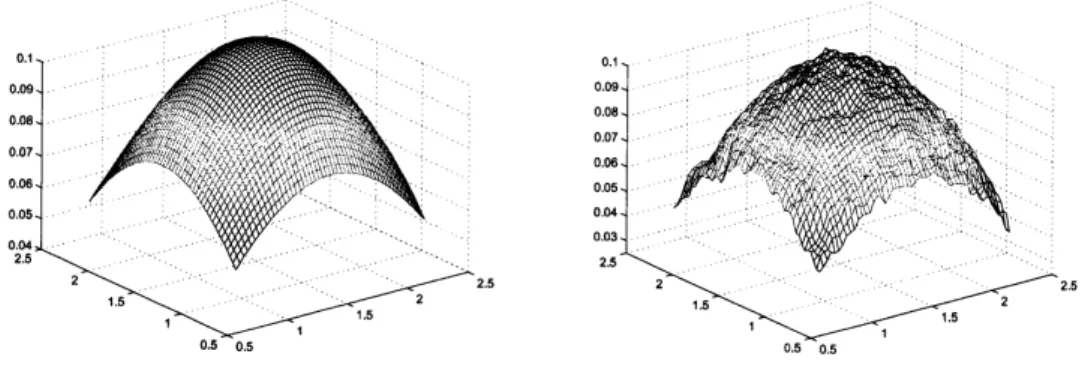
between $V_{k}^{(\ell)}$ and$v(t_{k}, S_{k}^{(\ell)}),$ _$\ell=1,$

$\ldots,$$N$, at $k=9$ is0.0064. Figure 1

compares $v(t_{k}, x)$ and

an

estimated value

function

using $V_{k}^{(\ell)\prime}s$ at $k=9$. We

use

the average

values

_of

$V_{k}^{(\ell)\prime}s$

in suitable clusters to estimate the value

_function

at

_uniform

$gnd$points. The

figure indicates that our method on the whole

underestimates

the analytical solution. This may

be because the number

_of

Monte Carlopaths shooting$\eta_{i}^{h}(t_{k}, S_{k}^{(\ell)}, a)/\lambda(h)$ ’s is still

insufficient.

Figure 1: The analytical (left) and estimated (right) value functions at $t=0.09$ around $x=$

$(\pi/2, \pi/2)^{*}.$

Acknowledgements

The author is thankful to Takashi Tamura for helpful comments. This study is partially

(9)

References

[1] G. Barles and P. E. Souganidis. Convergence of approximation schemes forfullynonlinear

second order equations. Asymptot. Anal., 4:271-283,

1991.

[2] F. Bonnans, E. Ottenwaelter, andH. Zidani. A fast algorithm for thetwodimensional HJB

equationof stochastic control. Math. Model. Numer. Anal., 38:723-735,

2004.

[3] F. Bonnans and H. Zidani. Consistency of generalized finite difference schemes for the

stochastic HJB equation.

SIAM

J. Numer. Anal., 41:1008-1021,

2003.

[4] B. Bouchard and N. Touzi. Discrete-time approximation and Monte

Carlo

simulation of

backward stochastic differentialequations. Stochastic Process. Appl., 111:175-206,

2004.

[5] F. Camilli and M. Falcone. An approximationscheme for the optimal control of diffusion

processes. Math. Model. Numer. Anal., 29:97-122,

1995.

[6] E. Carlini, M. Falcone,andR. Ferretti. An efficient algorithm for

Hamilton-Jacobi

equations

in high dimension. Comput. Visual. Sci., 7:15-29,

2004.

[7] K. Debrabant andE. R. Jakobsen. Semi-Lagrangianschemes forlinearandfully non-linear

diffusion equations. Math. Comp. to appear.

[8] A. Fahim, N. Touzi, and X. Warin. A probabilistic numerical method for fully nonlinear

parabolic PDEs. Ann. Appl. Probab., 21:1322-1364,

2011.

[9] W. H. Fleming and H. M. Soner. Controlled Markov pmcesses and viscosity solutions.

Springer-Verlag, NewYork, 2nd edition, 2006.

[10]

S. Graf

and H. Luschgy. Foundation

of

quantization

_for

pmbability distributions.

Springer-Verlag, Berlin,

2000.

[11] L. Gy\"orfi, M. Kohler, A. Krzyzak, andH.Walk. A

_{distribution-free}

theory

_of

nonpammetric

regression. Springer-Verlag, NewYork,

2002.

[12] N. V. Krylov. Controlled

_diffusion

processes. Springer-Verlag, New York,

1980.

[13] H. J. Kushner and P. Dupuis. Numencal methods

_for

stochastic control pmblems in

con-tinuous time. Springer-Verlag, New York, 2001.

[14] J.-P.Lemor, E.Gobet,and X. Warin. Rate ofconvergence of

an

empiricalregression method

for solving generalized backward stochastic differential equations. Bemoulli, 12:889-916,

2006.

[15] F. A. Longstaff and E. S. Schwartz. Valuing american options by simulation: a simple

least-squares approach. Rev. Finan. Stud., 14:113-147, 2001.

[16] Y. Nakano. An approximation scheme for optimal stochastic control problems. preprint,

(10)

[17] G. Pag\‘es, H. Pham, and J. Printems. An optimal Markovian quantization algorithm for

multidimensional stochastic control problems. Stoch. Dyn., 4:501-545, 2004.

[18] G. Pag\‘es and J.Printems. Optimal quadraticquantizationfor numerics: theGaussiancase.

Monte Carlo Methods Appl., 9:135-168,

2003.

[19] H. Pham.

Continuous-time

stochastic control and optimization with

_financial

applications.

Springer, Berlin,

2009.

Graduate

School

of

Innovation

Management

Tokyo

Institute

of Technology

2-12-1 W9-117 Ookayama 152-8552, Tokyo, Japan

$E$-mailaddress: [email protected]

$HI_{5\backslash }I\ovalbox{\tt\small REJECT} 2$ _シ$\exists\sqrt[\backslash ]{}Vj?\backslash \sqrt[\backslash ]{}\nearrow^{\backslash }\}\backslash \varpi f^{p}n^{t}H^{\backslash }\backslash$