Bounds for effective speeds of traveling fronts in spatially periodic media (Conference on Dynamics of Patterns in Reaction-Diffusion Systems and the Related Topics)

(1)

Bounds for effective speeds of

traveling

fronts

in

spatially periodic media

中村健一 (電気通信大学)

KEN-ICHI

NAKAMURA

Department ofComputer Science

The University ofElectrO-Communications

nakamura@im.uec.ac.jp

1. INTRODUCTION

We consider the following reaction-diffusion-advection equation

on

$\mathbb{R}$:

(1.1) $u_{t}= \epsilon u_{xx}+\epsilon b(x)u_{x}+\frac{1}{\epsilon}f(u)$, $x\in \mathbb{R}$, $t>0$,

where$\epsilon$isasmallpositive parameter, $b$is asmoothperiodic function withzeromean,

and $f(u)=-W’(u)$ is asmooth functionderived fromadouble-well potential$W(u)$

having different depth at its two wells. In the

case

where $b(x)\equiv 0$, it is

well-known that there exists atraveling front solution which travels at aconstant speed

preserving its shape ([3]). On the other hand, if $b(x)\not\equiv 0$, then traveling front

solutions in the usual sense can no longer exist. However, under suitable conditions

on $b$and $f$, thereexists akind offront solutions whoseshape and propagation speed

vary periodically in time ([8, 9]). Our aim in this article is to study the influence of

spatial inhomogeneity

on

the speed of front propagation inperiodic diffusive media.

Equation (1.1) is related to problems

on

front propagation in an infinite tubular

domain with asmooth and oscillating boundary. Let

$\Omega_{\sigma}=\{(x, \sigma y_{1}, \ldots, \sigma y_{n-1})\in \mathbb{R}\mathrm{x} \mathbb{R}^{n-1}|y=(y_{1}, \ldots, y_{n-1})\in\omega(x)\}$,

where $\sigma>0$ is aparameter and the map $x\mapsto\{v(x)$ is periodic. Matano [6] has

considered the Allen-Cahn equation

(1.2) $u_{t}= \epsilon\Delta u+\frac{1}{\epsilon}f(u)$, $x\in\Omega_{\sigma}$, $t>0$

under the homogeneous Neumann boundary conditions on $\partial\Omega_{\sigma}$ and has obtained

some conditions on $f$ and $\omega(x)$ for the existence and non-existence of traveling

fronts for (1.2). Some numerical experiments imply that the characteristics of front

propagation such as front speeds and front profiles

are

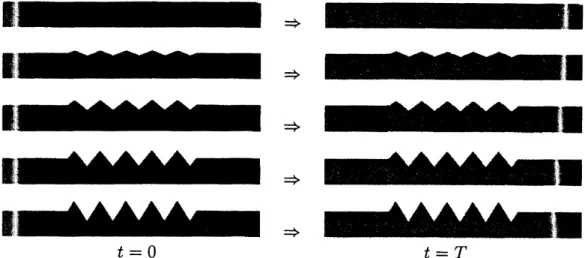
strongly influenced by the

shape of$\partial\Omega_{\sigma}$ (See Figure 1). It follows from an argument in [4] that equation (1.2

数理解析研究所講究録 1330 巻 2003 年 79-87

(2)

is formally reduced in the li mit $\sigmaarrow 0$ to equation (1.1) with $b(x)=a’(x)/a(x)$,

where $a(x)>0$ is the (n $-1)$-dimensional _{volume of}$\omega(x)$.

$\Rightarrow$ $\Rightarrow$ $\Rightarrow$ $\Rightarrow$ $\Rightarrow$ $t=0$ $t=T$

FIGURE 1. Numerical simulations of front propagation for (1.2) in

five different domains when $\epsilon=0.050$, $f(u)=u(1-u)(u-1/4)$

.

The

white region approximately represents the position of the front.

Since the effects ofdiffusion and advection

are

negligible for small $\epsilon$, the solution

of (1.1) is known to develop transition layers connecting two stable states within a

short ti me. Let $P^{\epsilon}(t)$ denote the position of

one

of the layers at time $t$

.

When the

parameter $\epsilon$ is small, we will

see

that the speed of the layer at time $t$has the formal

expansion

(1.3) $\frac{dP^{\epsilon}}{dt}=c-\epsilon b(P^{\epsilon})-\epsilon^{2}\gamma b’(P^{e})+$(higher order terms),

where $c>0$ is the speed of the traveling front solution in the homogeneous case

and $\gamma$ is

some

constant. By constructing suitable supersolutions and subsolutions

of (1.1), we justify the above formal expansion up to $\epsilon^{2}$

, provide sharp estimates

for the propagation speed of the front solution and show that spatial inhomogeneity

slows down the speed of front propagation for (1.1).

2. MAIN RESULT

Our hypotheses are

as

follows:

(B1) $b(x)$ is asmooth periodic function with least period $L>0$; (B2) $\int_{0}^{L}b(x)dx=0$;

(3)

(F1) $f$ is smooth and has exactly three

zeros

0,$\alpha$, 1 with $0<\alpha<1$;

(F2) $f(u)<0$ for $u\in(0, \alpha)\cup(1, +\infty)$, $f(u)>0$ for $u\in(-\infty, 0)\cup(\alpha, 1)$; (F3) $f’(0)<0$, $f’(1)<0$;

(F4) $\int_{0}^{1}f(u)du>0$.

Atypical example of$f$ is acubicfunction $f(u)=u(1-u)(u-\alpha)$ where$0<\alpha<1/2$

.

Inwhat follows

we

denote by $\langle g\rangle$ the

mean

of

an

-periodic function

$g$

on

$\mathbb{R}$, namely,

$\langle g\rangle=\frac{1}{L}\int_{0}^{L}g(x)dx$

.

In the homogeneous

case

$(b(x)\equiv 0)$, there exists atraveling front solution of(1.1)

written in the form

$u(x, t)=\phi$ $( \frac{x-d}{\epsilon})$

where $(\phi(\xi), c)$ is aunique solution of

(2.1) $\{$

$\phi_{\xi\xi}+c\phi_{\xi}+f(\phi)=0$, $\xi\in \mathbb{R}$

$\phi(-\infty)=1$, $\phi(0)=\alpha$, $\phi(+\infty)=0$

.

In addition, the speed $c$ is positive by virtue of (F4). See [3] for details.

In the periodic

case

$(b(x)\not\equiv 0)$, the notion oftraveling fronts has to be replaced

as follows:

Definition. Asolution $U^{e}$ of (1.1) satisfying

(2.2) $\lim_{xarrow-\infty}U^{\epsilon}(x, t)=1$, $\lim_{xarrow+\infty}U^{\epsilon}(x, t)=0$ for all $t\in \mathbb{R}$

is called atraveling front if there exists a $T_{\epsilon}>0$ such that

(2.3) $U^{\epsilon}(x, t+T_{\epsilon})=U^{\epsilon}(x-L, t)$ for all $x\in \mathbb{R}$, $t\in \mathbb{R}$

.

We define the effective speed (or the average speed) $s_{\epsilon}$ of$U^{\epsilon}$ by $L/T_{\epsilon}$

.

The main result of this article is:

Theorem 1. Suppose that $b(x)\not\equiv 0$

.

Then there exist positive constants $\epsilon_{0}$ and $C$

such that

_for

any $\epsilon\in(0, \epsilon_{0})$, we have

(2.4) $|s_{\epsilon}-(c- \frac{\langle b^{2}\rangle}{c}\epsilon^{2})|\leq C\epsilon^{3}|\log\epsilon|^{2}$

.

Thus spatial inhomogeneity slows down the

_front

propagation in this case.

Remark 2. Some existenceresults fortravelingfronts ofmultidimensional

reaction-diffusion-advectionequations withbistable nonlinearities have been obtainedby Xin

$[8, 9]$ onthe suppositionthatdiffusion and advectioncoefficients

are

nearlyconstant

(4)

Applying his results to (1.1), we see that if $\epsilon$ is sufficiently small there exists a

traveling front $U^{\epsilon}$ satisfying (2.2) and (2.3) with positiveeffective

speed $s_{\epsilon}$ and that

it is unique up to time shift.

Remark 3. In [5], Heinze, Papanicolaou and Stevens has given

_some

variational

formulas of the effective speeds of traveling fronts in the multidimensional case.

However, it is rather difficult to obtainsharp estimates for $s_{\epsilon}$ like (2.4) by using the

formulas.

3. FORMAL ASYMPTOTIC EXPANSIONS OF THE FRONT SPEED

In this section we present _{aformal derivation of} the propagation speed of the

traveling front $U_{\epsilon}$ for (1.1).

Suppose that equation $U^{\epsilon}(x, t)=\alpha$ has aunique solution _{$x=P^{\epsilon}(t)$} for each $t$

and that $U^{\epsilon}$ and $P^{\epsilon}$ have the expansions

$U^{\xi}(x, t)=U_{0}(\xi, t)+\epsilon U_{1}(\xi, t)+\epsilon^{2}U_{2}(\xi, t)+\cdots$ ,

(3.1)

$P^{\epsilon}(t)=P_{0}(t)+\epsilon P_{1}(t)+\epsilon^{2}P_{2}(t)+\cdots$ ,

where $\xi$ _{$=(x-P^{\epsilon}(t))/\epsilon$}

.

The stretched space variable

$\xi$ gives the right spatial

scaling to describe the sharptransition layer between the two stable states 0and 1.

Since $U^{\epsilon}=\alpha$ at $P^{\epsilon}(t)$,

we

normalize $U_{k}$ in such away that

(3.2) $U_{0}(0, t)=\alpha$, $U_{k}(0,t)=0$ (A _$=1,2$, $\ldots$)

for all $t$ (normalizationconditions). By (2.2),

we

alsoimpose

the following conditions

as $\xiarrow\pm\infty$:

(3.3) $U_{0}(-\infty, t)=1$, $U_{0}(+\infty, t)=0$, _{$U_{k}(\pm\infty, t)=0(k=1,2, \ldots)$}

for all $t$ (limiting conditions).

Substituting the above expansions (3.1) into (1.1) and collecting the $\epsilon^{0}$ terms, we

obtain

$U_{0\xi\xi}+P_{0t}U_{0\xi}+f(U_{0})=0$

.

From this together with (3.2) and (3.3), we find that

$U_{0}(\xi, t)=\phi(\xi)$, $P_{0t}=c$,

where $(\phi, c)$ is the unique solution of (2.1).

Collecting the $\epsilon^{1}$ terms and recalling

(3.2) and (3.3),

we

get

(3.4) $\{$

$U_{1\xi\xi}+cU_{1\xi}+f’(\phi(\xi))U_{1}=-(P_{1\mathrm{t}}+b(P_{0}))\phi’(\xi)$, $\xi\in \mathbb{R}$,

$U_{1}(-\infty, t)=0$, $U_{1}(0, t)=0$, $U_{1}(+\infty, t)=0$

.

The following Fredholmtype lemmagives

_us

thesolvabilityconditions for (3.4). For

the case $c=0$, similar statements have been appeared in [1]

(5)

Lemma 4. Let $A(\xi)$ be given and assume that $A(\xi)=O(e^{-\mu|\xi|})$ as $|\xi|arrow\infty$

for

some $\mu>0$. Then thefollowing problem

$\{$

$\Psi_{\xi\xi}+c\Psi_{\xi}+f’(\phi(\xi))\Psi=A(\xi)$, $\xi\in \mathbb{R}$,

$\Psi(0)=0$,

has a bounded solution

_if

and only

_if

$\int_{\mathrm{R}}A(\xi)\phi’(\xi)e^{c\xi}d\xi=0$.

Moreover, the solution is written by

$\Psi(\xi)=\phi’(\xi)\int_{0}^{\xi}\phi’(y)^{-2}e^{-cy}\{\int_{-\infty}^{y}A(z)\phi’(z)e^{cz}dz\}dy$,

and

_satisfies

$\Psi(\xi)$, $\Psi’(\xi)$, $\Psi$’$’(\xi)=O(e^{-\mu|\xi|})$

as

$|\xi|arrow\infty$

.

By this Lemma, the solvability condition for (3.4) yields $P_{1t}=-b(P_{0})$ and thus

$U_{1}(\xi, t)=0$ for all $(\xi, t)$

.

In the

same

way as above, collecting the $\epsilon^{2}$ terms,

we

get

(3.5) $\{$

$U_{2\xi\xi}+cU_{2\xi}+f’(\phi(\xi))U_{2}=-(P_{2t}+b’(P_{0})(P_{1}+\xi))\phi’(\xi)$, $\xi\in \mathbb{R}$,

$U_{2}(-\infty, t)=0$, $U_{2}(0, t)=0$, $U_{2}(+\infty, t)=0$

.

Again by Lemma 4, the solvability condition for (3.5) yields

$P_{2t}=-b’(P_{0})(P_{1}+\gamma)$, $U_{2}(\xi, t)=b’(P_{0}(t))V(\xi)$,

where $\gamma$ $\in \mathbb{R}$ is defined by

$\gamma=\frac{\int_{1\mathrm{R}}\phi’(\xi)^{2}e^{c\xi}\xi d\xi}{\int_{\mathrm{R}}\phi’(\xi)^{2}e^{c\xi}d\xi}$ ,

and

$V( \xi)=\phi’(\xi)\int_{0}^{\xi}\phi’(y)^{-2}e^{-cy}\{\int_{-\infty}^{y}(\gamma-z)\phi’(z)^{2}e^{cz}dz\}dy$

.

Consequently, we obtain the following formal asymptotic expansions

(3.6) $U^{\epsilon}(x, t)= \phi(\frac{x-P^{\epsilon}(t)}{\epsilon})+\epsilon^{2}b’(P^{\epsilon}(t))V(\frac{x-P^{\epsilon}(t)}{\epsilon})+\cdots$ ,

and

$\frac{dP^{e}}{dt}=c-\epsilon b(P_{0}(t))-\epsilon^{2}b’(P_{0}(t))(P_{1}(t)+\gamma)+\cdots$ ,

(3.7)

$=c-\epsilon b(P^{\epsilon}(t))-\epsilon^{2}\gamma b’(P^{\epsilon}(t))+\cdots$

.

(6)

4. PRELIMINARIES

Let $\delta_{0}>0$ be such that for each $\delta\in[-\delta_{0}, \delta_{0}]$, _{$f_{\delta}(u)=f(u)+\delta$} satisfies the

following conditions:

(a) $f_{\delta}$ has exactly three

zeroes

$\zeta_{0}(\delta)$,$\zeta_{\alpha}(\delta)$, $\zeta_{1}(\delta)$ with $\zeta_{0}(\delta)<\zeta_{\alpha}(\delta)<\mathrm{C}\mathrm{i}(6)$;

(b) $f_{\delta}’(\zeta_{0}(\delta))<0$, $f_{\delta}’(\zeta_{\alpha}(\delta))>0$ and $f_{\delta}’(\zeta_{1}(\delta))<0$;

$( \mathrm{c})\int_{\zeta_{0}(\delta)}^{\zeta_{1}(\delta)}f_{\delta}(u)du>0$

.

Then there exists asolution $(\psi, s)=(\psi(\xi;\delta), s(\delta))$ of

(4.1) $\{$

$\psi_{\xi\xi}+s\psi_{\xi}+f_{\delta}(\psi)=0$, $\xi\in \mathbb{R}$,

$\psi(-\infty)=\zeta_{1}(\delta)$, $\psi(0)=\alpha$, $\psi(+\infty)=\zeta_{0}(\delta)$,

satisfying $\psi_{\xi}(\xi;\delta)<0$ for all $\xi\in \mathbb{R}$ and $s(\delta)>0([3])$

.

It is known that $\psi(\cdot;\delta)arrow\phi$

uniformly

on

$\mathbb{R}$ and $s(\delta)=c+O(\delta)$ as $\deltaarrow 0$, where _{$(\phi, c)$} is the solution of (2.1).

For $\delta\in[-\delta_{0}, \delta_{0}]$,

we

define afunction $V(\cdot;\delta)$ by

(4.2) $V( \xi;\delta)=\psi_{\xi}(\xi;\delta)\int_{0}^{\xi}\psi_{\xi}(\xi;\delta)^{-2}e^{-s(\delta)\eta}\{\int_{-\infty}^{\eta}(\gamma(\delta)-\zeta)\psi_{\xi}(\zeta;\delta)^{2}e^{s(\delta)\zeta}d\zeta\}d\eta$,

where

(4.3) $\gamma(\delta)=\frac{\int_{\mathrm{J}\mathrm{B}}\psi_{\xi}(\xi,\delta)^{2}e^{s(\delta)\xi}\xi d\xi}{\int_{\mathrm{R}}\psi_{\xi}(\xi\cdot\delta)^{2}e^{s(\delta)\xi}d\xi}.,\cdot$

Then the function $V(\cdot;\delta)$ solves the problem

(4.4) $\{$

$V_{\xi\xi}+s(\delta)V_{\xi}+f’(\psi(\xi;\delta))V=(\gamma(\delta)-\xi)\psi_{\xi}(\xi;\delta)$, $\xi\in \mathrm{R}$,

$V(0;\delta)=0$

.

Furthermore, $\psi(\xi;\delta)$ and $V(\xi;\delta)$ satisfy the following:

Lemma 5. There eist positive constants $M$ and Adepending

on

$\delta_{0}$ such that

if

$|\delta|\leq\delta_{0\prime}$ then

$\zeta_{1}(\delta)-Me^{\Lambda\xi}\leq\psi(\xi;\delta)<\zeta_{1}(\delta)$,

for

_{$\xi\leq 0$},

$\zeta_{0}(\delta)<\psi(\xi;\delta)\leq\zeta_{0}(\delta)+Me^{-\Lambda\xi}$,

for

$\xi\geq 0$,

(4.5) $-Me^{-\Lambda|\xi|}\leq\psi_{\xi}(\xi;\delta)<0$,

for

$\xi\in \mathbb{R}$,

$|\psi_{\xi\xi}(\xi;\delta)|\leq Me^{-\Lambda|\zeta|}$ ,

for

$\xi\in \mathbb{R}$, $|V(\xi;\delta)|$, $|V_{\xi}(\xi;\delta)|$, $|V_{\xi\xi}(\xi;\delta)|\leq Me$$-\Lambda|\xi|$,

for

$\xi\in \mathbb{R}$

.

(7)

5. CONSTRUCTION OF SUPERSOLUTIONS AND SUBSOLUTIONS

This section is devoted to the proof of Theorem 1. In order to obtain sharp

estimates for the effective speed $s^{\epsilon}$, we construct suitable supersolutions and

subs0-lutions of (1.1). The formal asymptotic expansions (3.6) and (3.7) provide us with

useful information for the construction.

Let $\psi(\xi;\cdot)$, $V(\xi;\cdot)$, $\zeta_{0}(\cdot)$, $\zeta_{1}(\cdot)$, $\gamma(\cdot)$ and $s(\cdot)$ be as in the previous section and

define $\phi_{\epsilon}^{\pm}(\xi)=\psi(\xi;\pm h\epsilon^{3})$, $V_{\epsilon}^{\pm}(\xi)=V(\xi;\pm h\epsilon^{3})$, $z_{j}^{\pm}(\epsilon)=\zeta_{j}(\pm h\epsilon^{3})(j=0,1)$, $\gamma_{\epsilon}^{\pm}=\gamma(\pm h\epsilon^{3})$ and $c_{\epsilon}^{\pm}=s(\pm h\epsilon^{3})$, where $h$ is apositive constant. In other words,

$(\phi_{\epsilon}^{\pm}, c_{\epsilon}^{\pm})$ and $V_{\epsilon}^{\pm}(\xi)$ satisfy

$\{$

$\frac{d^{2}\phi_{\epsilon}^{\pm}}{d\xi^{2}}+c_{\epsilon}^{\pm}\frac{d\phi_{\epsilon}^{\pm}}{d\xi}+f(\phi_{\epsilon}^{\pm})\pm h\epsilon^{3}=0$ , $\xi\in \mathbb{R}$, $\phi_{\epsilon}^{\pm}(-\infty)=z_{1}^{\pm}(\epsilon)$, $\phi_{\epsilon}^{\pm}(0)=\alpha$, $\phi_{\epsilon}^{\pm}(+\infty)=z_{0}^{\pm}(\epsilon)$,

and

$\{$

$\frac{d^{2}V_{\epsilon}^{\pm}}{d\xi^{2}}+c_{\epsilon}^{\pm}\frac{dV_{\epsilon}^{\pm}}{d\xi}+f’(\phi_{\epsilon}^{\pm})V_{\epsilon}^{\pm}=(\gamma_{\epsilon}^{\pm}-\xi)\frac{d\phi_{\epsilon}^{\pm}}{d\xi}$ , _{$\xi\in \mathbb{R}$},

$V_{\epsilon}^{\pm}(\pm\infty)=V_{\epsilon}^{\pm}(0)=0$,

respectively. In what follows we assume that $h\epsilon^{3}<\delta_{0}$, where $\delta_{0}$ is the positive

constant in the previous section.

Let $K$ be apositive constant and define functions $W_{\epsilon}^{\pm}$ by

(5.1) $W_{\epsilon}^{\pm}(x, t)= \phi_{\epsilon}^{\pm}(\frac{x-R_{\epsilon}^{\pm}(t)}{\epsilon})+\epsilon^{2}b’(R_{\epsilon}^{\pm}(t))V_{\epsilon}^{\pm}(\frac{x-R_{\epsilon}^{\pm}(t)}{\epsilon})$,

where $R_{\epsilon}^{\pm}$

are

solutions of

(5.2) $\frac{dR_{\epsilon}^{\pm}}{dt}=c_{\epsilon}^{\pm}-\epsilon b(R_{\epsilon}^{\pm})-\epsilon^{2}\gamma_{\epsilon}^{\pm}b’(R_{\epsilon}^{\pm})\pm K\epsilon^{3}|\log\epsilon|^{2}$.

Proposition 6. There eist positive constants $h$, $K$ and $\epsilon_{0}$ depending

on

$\delta_{0}$ such

that

_if

$\epsilon$ $\in(0, \epsilon_{0})$, then $W_{\xi}^{+}$ is a supersolution

of

(1.1) and $W_{\epsilon}^{-}$ is a subsolution

of

(1.1).

Outline

_of

proof. Weonlyshow that$W_{\epsilon}^{+}$ is asupersolutionof(1.1) since theassertion

for $W_{\epsilon}^{-}$

can

be proved in the

same manner.

In the rest of the proof, we drop the

subscript $\epsilon$ for simplicity. We define

(5.3) $I(x, t)=\epsilon^{2}W_{xx}^{+}+\epsilon^{2}b(x)W_{x}^{+}+f(W^{+})-\epsilon W_{t}^{+}$

and $\eta(x, t)=(x-R^{+}(t))/\epsilon$. Substituting (5.1) into (5.3),

we

get

$I(x, t)=-h\epsilon^{3}+\{R_{t}^{+}-c^{+}+\epsilon b(x)\}\phi_{\xi}^{+}(\eta)+f(\phi^{+}(\eta)+\epsilon^{2}b’(R^{+})V^{+}(\eta))-f(\phi^{+}(\eta))$

$+\epsilon^{2}b’(R^{+})V_{\mathrm{C}\mathrm{C}}(\eta)+\epsilon^{2}b’(R^{+})\{R_{t}^{+}+\epsilon b(x)\}V_{\xi}^{+}(\eta)-\epsilon^{3}b’(R^{+})R_{t}^{+}V(\eta)$

.

(8)

By Lemma 5, there exists apositive constant $\mu$ depending

on

$\delta_{0}$ satisfying $|\phi_{\xi}^{+}|$, $|V^{+}|$, $|V_{\xi}^{+}|$, $|V_{\xi\xi}^{+}|<\epsilon^{4}$ for $|\xi|>\mu|\log\epsilon|$.

Therefore, $I(x, t)=-h\epsilon^{3}+O(\epsilon^{4})<0$ for $|x-R^{+}(t)|>\mu\epsilon|\log\epsilon|$ when $\epsilon$ is small.

In the

case

where $|x-R^{+}(t)|\leq\mu\epsilon|\log\epsilon|$, we see that

$I(x, t) \leq\{K-\frac{\mu^{2}}{2}|b’(R^{+})|\}\phi_{\xi}^{+}\epsilon^{3}|\log\epsilon|^{2}-\{h-c|b’(R^{+})V^{+}|\}\epsilon^{3}+O(\epsilon^{4}|\log\epsilon|^{3})$

.

Since $\phi_{\xi}^{+}<0$, if$h>\mu^{2}||b’||_{\infty}/2$and $K>cM||b’||_{\infty}$, then$I(x, t)<0$for small$\epsilon$

.

$\square$

Corollary 7. Fix $\epsilon\in(0, \epsilon_{0})$

.

Tften for

any $t\in \mathbb{R}$,

we

have

$\inf_{x\in \mathbb{R}}W_{\epsilon}^{+}(x, t)>0$,

$\sup_{x\in \mathrm{R}}W_{\epsilon}^{-}(x, t)<1$

.

Since the right-hand sides of (5.2)

are

$L$-periodic and positive for small $\epsilon$, there

exist positive constants $\tau_{\epsilon}^{\pm}$ satisfying

(5.4) $R_{\epsilon}^{\pm}(t+\tau_{\epsilon}^{\pm})=R_{\epsilon}^{\pm}(t)+L$

for all $t\in \mathbb{R}$.

Let $x_{0}$ be such that $U^{\epsilon}(x_{0},0)=\alpha$

.

By (2.2) and Corollary 7, we can choose $R_{\epsilon}^{-}(0)<x_{0}<R_{\epsilon}^{+}(0)$ such that

$W_{\epsilon}^{-}(x, \mathrm{O})\leq U^{\epsilon}(x, 0)\leq W_{\epsilon}^{+}(x, 0)$

.

Hence the comparison theorem yields that

$W_{\epsilon}^{-}(x, t)<U^{\zeta}(x, t)<W_{\epsilon}^{+}(x, t)$

for all $t>0$

.

Thus we obtain:

Lemma 8. Let $s_{\epsilon}=L/T_{\epsilon}$ be the

effective

speed

of

$U^{\epsilon}$

.

Then $L/\tau_{\epsilon}^{-}\leq s_{\epsilon}\leq L/\tau_{\epsilon}^{+}$

.

Proof

of

Theorem 1. Let $A_{\epsilon}^{\pm}=c_{\epsilon}^{\pm}\pm K\epsilon^{3}|\log\epsilon|^{2}$ and $B_{\epsilon}^{\pm}(R)=\epsilon b(R)+\epsilon^{2}\gamma_{\epsilon}^{\pm}b’(R)$

.

Then it follows from (5.2) and (5.4) that

$\frac{L}{\tau_{\epsilon}^{\pm}}=\frac{1}{\langle(A_{\epsilon}^{\pm}-B_{\epsilon}^{\pm}(\cdot))^{-1}\rangle}$ .

Since $A_{\epsilon}^{\pm}=c.+O(\epsilon^{3}|\log\epsilon|^{2})$and since $B_{\epsilon}^{\pm}$ are -periodic functions with $\langle B_{\epsilon}^{\pm}\rangle=0$,

$\langle(A_{\epsilon}^{\pm}-B_{\epsilon}^{\pm}(\cdot))^{-1}\rangle=\frac{1}{c}(1+\frac{\langle b^{2}\rangle}{c^{2}}\epsilon^{2}+O(\epsilon^{3}|\log\epsilon|^{2}))$ ,

and hence

(5.5) $\frac{L}{\tau_{\epsilon}^{\pm}}--c-\frac{\langle b^{2}\rangle}{c}\epsilon^{2}+O(\epsilon^{3}|\log\epsilon|^{2})$

.

The assertion of the theorem immediately follows from (5.5) and Lemma 8.

0

(9)

REFERENCES

[1] N. D. Alikakos, P. W. Bates and X. Chen, Convergence _ofthe Cahn-Hilliard equation to the

Hele-Show model, Arch. Rational Mech. Anal., 128 (1994), 165-205.

[2] H. Berestycki and F. Hamel, Front propagation in periodic excitable media, Comm. Pure

Appl. Math., 55 (2002), 949-1032.

[3] P. C. Fife and J. B. McLeod, The approach _ofsolutions _ofnonlinear _diffusion equations to

traveling_frontsolution, Arch. Rational Mech. Anal., 65 (1977), 335-362.

[4] J. K.Hale andG. Raugel,_{Reaction-diffusion} equation on thindomains, J. Math. Pures Appl.

71 (1992), 33-95.

[5] S. Heinze, G. Papanicoiaou and A. Stevens, Variational Principle _forpropagation speeds in

inhomogeneous media, SIAM Appl. Math., 62 (2001), 129-148.

[6] H. Matano, Applied Analysis Seminar, Univ. ofTokyo, 1995;EcoleNormale Sup\’erieure Sem-inar, 1996.

[7] K. I. Nakamura, _Effective speed _oftravelling _wavefronts in inhomogeneous media,

Proceed-ings ofthe Workshop “Nonlinear Partial Differential Equations and Related Topics”, Joint

Research Center for Scienceand TechnologyofRyukoku University, 53-60, 1999.

[8] X. Xin, Existence and stability _oftravelling waves inperiodic media governed by a bistable

nonlinearity, J. Dyn. Diff. Eq., 3(1991), 541-573.

[9] J. X. Xin, Eistence and nonexistence _oftraveling waves and _{reaction-diffusion}_front$P\gamma vpa-$ gation in periodic media, J. Statist. Phys., 73 (1993), 893-926.

[10] J. Xin, $fi$}_$vnt$propagation inheterogeneous media, SIAM Review, 42 (2000), 161-230