Characterization of a Chaotic Economic Dynamics by Unstable Periodic Solutions : An Application to a Generalized Goodwin Model (Mathematical Economics)

Characterization of aChaotic Economic

Dynamics

by

Unstable Periodic

Solutions

-An Application to aGeneralized Goodwin Model*

Ken-ichi Ishiyama\dagger _{, Yoshitaka Saiki}\ddagger

Department of Mathematical Sciences

Graduate School of Mathematical Sciences, University of Tokyo

3-8-1 Komaba, Meguro, Tokyo 153-8914, Japan

Abstract

In this paperwestudy the propertiesof the chaotic behavior in agrowthcycle model and the unstableperiodicsolutions foundin the attractor, and therebywepoint outsome

similarities between them. This attempt comes from the recent work in physics. The

result implies unstable periodic solutions can be the keywords to understand the chaotic dynamics.

1Introduction

It is

no

doubt the analysis of the growth trajectory in aphase space

is

one

of the most important themes in economic dynamics. It is often

discussed what happens when agrowth cycle model has been extended

in adirection. In particular, atopic has attracted much attention since

$1980\mathrm{s}$, that is, the controversy surrounding the effects of fiscal policy

on

asimple trade cycle(W01fstetter(1982), Goodwin(1990), Takamasu(1995),

Yoshidaand Asada(2001)$)$

.

Howeverlike

as

other topics there

are

also few

works concerning this point in which the comparativedynamics involving

the chaotic behavior is discussed.

In recent work in physics(Zoldi and Greenside(1998), Kawahara and

Kida(2001), Kato and Yamada(2002)$)$, anumerical approach has been

attempted using unstable periodic solutions to explain typical chaotic

be-havior and statistical properties in chaotic solutions. The main purpose

of this paper is to propose

an

idea analogous to physics to understand the

dynamics of achaotic business cycle, which

can

be expected to be useful

to clarify various chaotic phenomena shown in economic dynamics.

$.\mathrm{W}\mathrm{e}$aregratefulto Professor T. Fujimotoand Professor M. Yamadafortheiruseful comments and fruitful

discussions. The authors retain allresponsibilityforremainingerrorsand omissions.

$\uparrow E$-rnail:ishiyama@ms.

$\mathrm{u}$-tokyo.$\mathrm{a}\mathrm{c}.$jp $\iota_{E}$-rnail:8aiki\copyright ms.

$\mathrm{u}$-tokyo.ac.jp

数理解析研究所講究録 1337 巻 2003 年 92-102

The plan of this paper is

as

follows. In the next section, we give an

example of the nonlinear macr0-economic model. Section 3describes

the properties of the dynamics of the model, where the characteristics

of achaotic solution and unstable periodic solutions are illustrated. It

is cleared in section 4that the chaotic behavior in the dynamics of the

model is qualitatively and quantitatively related to the unstable periodic

solutions found in the attractor. In the final section,

we

conclude

our

results and state the possibility of the application.

2The Model

First, we propose agrowth cycle model

as

an

example which represents

a

chaotic behavior caused by asimple interaction between countries. The

model is based

on

Goodwin(1967) and its extensions. It consists of

fol-lowing assumptions.

(A1) We consider twocountries, where there exist respectively three agents:

the government, capitalists, and workers. These countries

are

al-most homogeneous, but parameters regarding astabilization policy

assumed next

can

be different.

(A2) The government controls the public expenditure

as

acountercyclical

policy, while it is financed by income tax and bond selling. The level

of the public expenditure is decided

on

the basis of two factors: the

scale ofthe domestic industry and the domestic employment

rate.l

(A3) The foreign capital share rate

as

well

as

the domestic capital share

$\mathrm{r}\mathrm{a}\mathrm{t}\mathrm{e}^{2}$

concern

the amount of

investment in each individual country.

This is the only mutual interaction allowed for in the model. The

invested capital and the labor employed contribute to the

produc-tion activity in each country. The level of employment is linearly

dependent

on

the scale of the production.

(A4) The workers bargain with capitalists for their money wages rate

tak-ing into consideration of the expected rate of inflation. Moreover the

bargaining power is influenced by the employment $\mathrm{r}\mathrm{a}\mathrm{t}\mathrm{i}\mathrm{o}.3$

(A5) The workers spend their whole disposable incomes, while the

cap-italists

save

their interest incomes besides the better part of their

lSeeWolfstetter(1982).

$2\mathrm{I}\mathrm{f}$we$\mathrm{c}\mathrm{o}\mathrm{n}8\mathrm{i}\mathrm{d}\mathrm{e}\mathrm{r}$the profitrateinstead of the

caPitalshare rate withinternationaltrade,thediscussionbecomes

extremelydIfficult.

$3\mathrm{A}\mathrm{n}$expectation-augmented wagePhillipscurve

isconsideredasYoshida and Asada(2001).

profits. The saving is devoted to the investment otherwise

purchas-ing the government bond.

(A6) The population and the productivity per capita grow with constant

rates. The price is rigid, that is to say, the gradient of change in price

is gentler than that of change in unit labor cost of $\mathrm{o}\mathrm{u}\mathrm{t}\mathrm{p}\mathrm{u}\mathrm{t}.4$

(A7) The growth of the national output depends

on

the relationship

be-tween the demand and the supply. For convenience, the

excess

supply

is consumed by capitalists, hence the aggregate output is equal to the

aggregate income.

From above assumptions,

we

construct the model which describe the

in-teraction among the labor share rates, the employment ratios, and the

expected inflation rates in two countries.

We formulate in advance the six-dimensional simultaneous ordinary

differential equations to be derived

as

follows:

$\frac{du_{i}}{dt}=(\hat{w}_{i}-(\alpha+\hat{p}_{i}))u_{i}$, (1)

$\frac{dv_{i}}{dt}=(\hat{\mathrm{Y}}_{i}-(\alpha+\beta))v_{i}$, (2)

$\frac{d\pi_{i}^{e}}{dt}=\theta(\hat{p}_{i}-\pi_{i}^{e})$, (3)

$i=1,2$,

where the variable $u_{i}$

means

the labor share rate in

$i$-th country,

$v_{i}$ the

employment ratio, and $\pi_{i}^{e}$ the expected rate of inflation respectively. The

constant $\gamma$ corresponds to the price rigidity assumed in (A6),

$\alpha$ the rate

of the technical

progress,

$\beta$ the growth rate of labor available, and 0is

aparameter with respect to the adaptive behavior of the worker. The

symbols $\hat{w}_{i},\hat{p}_{i}$, and $\hat{\mathrm{Y}}_{i}$

represent the respective change rates of the money

wage, of the price of goods, and of the national output in $i$-th country.

They are summarized or rewritten as follows:

$\hat{w}_{i}=f_{i}(v_{i}, \pi_{i}^{e})$; $\frac{\partial f_{i}}{\partial v_{i}}>0,$ $\frac{\partial f_{i}}{\partial\pi_{i}^{e}}>0$, (4)

$\hat{p}_{i}=\gamma(\hat{w}_{i}-\alpha)$, (5)

$4\mathrm{W}\mathrm{e}$considerthepriceadjustment equationassumedin Desai(1973) withaconstant mark-upfactor.

$\epsilon\hat{\mathrm{Y}}_{i}=h_{i}(u_{1}, u_{2})+(1-c)\mu_{i}(v^{*}-v_{i})+(\delta-1)(1-c)(1-u_{i})$ , (6)

where the right-hand side in equation(6) corresponds to the

excess

de-mand5

per output, while $\epsilon,$ _$c,$ $\delta,$ $v^{*}$, and $\mu_{i}$ are respectively

an

output

adjustment coefficient, the consumption coefficient of capitalists, the

in-come

tax rate, the target employment rate set so that $f(v^{*}, 0)=\alpha$, and

the parameter of fiscal policy in $i$-th country. The function $h_{i}$ determine

the effect of the investment on the augmentation of the $\mathrm{o}\mathrm{u}\mathrm{t}\mathrm{p}\mathrm{u}\mathrm{t}.6$ It has

the following properties:

$\frac{\partial h_{\dot{l}}}{\partial u_{i}}<0,$ $\frac{\partial h_{i}}{\partial u_{j}}>0$; $i,j=1,2$ $(j\neq i)$.

In the next section,

we

will discuss numerically the properties of the

solution of the model for aspecific

case.

3The Chaotic Solution and the Unstable Periodic Solutions

In this section weconsider characteristics of the solutions of the model for

aset of parameters and specified $\mathrm{f}\mathrm{u}\mathrm{n}\mathrm{c}\mathrm{t}\mathrm{i}\mathrm{o}\mathrm{n}\mathrm{s}.7$ Here we give two functions

based

on

Yoshida and Asada(2001):

$f_{i}(v_{i}, \pi_{i}^{e})=0.1(\frac{1}{1-v_{i}}-4.8)+\pi_{i}^{e}$, (7)

$h_{i}(u_{1},u_{2})=1.5(1-u_{i})^{5}-10.0(u_{i}-u_{j})^{3}$, (8)

while

we

set constants and parameters

as

$\alpha=0.02,$ $\beta=0.01,$ $\gamma=0.5$,

$\theta=0.8,$ $\epsilon=10.0,$ $\mathrm{c}=0.3,$ $\delta=\frac{2}{7},$ $v^{*}=0.8;\mu_{1}=1.2,$ and $\mu_{2}=8.0$

.

Note that the inequality $\mu_{1}<\mu_{2}$

means

that the government in country 2

takes

more

positive stabilizing policy than the other, and the interaction

between countries is represented by the second term in equation(8).

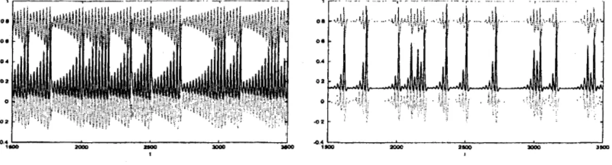
The time series after the transition is plotted in Fig. 1, where the

econ-omy

sustained by

more

positive fiscal policy looks stable for along time

but sometimes disturbed by the other country. The oscillations in two

countries

seem

to be synchronizedby the interaction inequation(8).

More-over

it is observed in this figure that the business tides, which

seem

repeated $\mathrm{r}\mathrm{e}\mathrm{g}\mathrm{u}1\mathrm{a}\mathrm{r}1\mathrm{y}^{8}$, tend to become gradually larger and suddenly get $\epsilon \mathrm{I}\mathrm{t}$includesthegovernmentexpenditure$G=\delta Y+\mu(v^{*}-v)Y$.

$\epsilon \mathrm{I}\mathrm{t}$

is basedonSkott(1989).

$7\mathrm{F}\mathrm{o}\mathrm{r}$some

parametersettings, wehave derived qualitatively similar results.

$8\mathrm{I}\mathrm{t}$

isabout 23 yearsin length forourparametersetting.

smaller. We

can

view each trend from expansion to contraction as

achar-acteristic cycle in each country. Hereafter

we

call the individual trend

economic $regime.9$ There appear $\mathrm{f}\mathrm{o}\mathrm{u}\mathrm{r}\mathrm{t}\mathrm{e}\mathrm{e}\mathrm{n}1$ economic regirnes in Fig.1.

We notice they have different length. Fig.2 shows asequence of economic

regimes

as

regarding the labor share rate and the employment ratio in

country 1. The pattern consisting of them looks like atmmpet chain.

Fig. 1: Time seriesin country $1(\mathrm{l}\mathrm{e}\mathrm{f}\mathrm{t})$ andcountry $2(\mathrm{r}\mathrm{i}\mathrm{g}\mathrm{h}\mathrm{t})$

The solid line is atime series of the labor sharerate, the dashed linethe employment ratio,

and the dotted line theexpected rate of inflation respectively. The horizontal axismeans the

time. Inour parameter setting, the unit time approximately equals ayear.

Fig. 2: Trajectory like atreernpet chain

Acyclical growth path ofthe labor sharerate$u_{1}$ and the employment ratio $v_{1}$ isillustrated.

Besides the chaotic solution,

we

have found thirteen kinds of periodic

$\mathrm{s}\mathrm{o}\mathrm{l}\mathrm{u}\mathrm{t}\mathrm{i}\mathrm{o}\mathrm{n}\mathrm{s}.12$

These

are

not stable, however,

we presume

the economy

suf-ficiently close such asolution

grows

along the trajectory for along time.

In the literatures of mathematics and physics, they

are

called unstable

periodic orbits(UPOs), and there is

an

idea that unstable periodic orbits

$9\mathrm{I}\mathrm{n}$

meteorology, the typical dynamicsarecalled weather$l\epsilon g|me$.

$10\mathrm{T}\mathrm{h}\mathrm{e}$last

$\mathrm{p}\mathrm{r}\mathrm{o}\mathrm{c}\infty \mathrm{s}$ofexPansionis not counted because of itsincomPletenae8.

llWeconsider the solution$X$is periodic if $||X(T)-X(0)||\leq 10^{-5}$,where$T$isthe period.

$12\mathrm{S}\mathrm{u}\mathrm{r}\mathrm{p}\mathrm{r}\mathrm{i}\mathrm{s}\mathrm{i}\mathrm{n}\mathrm{g}\mathrm{l}\mathrm{y}$we have observed every economic

regimes associatingevery unstableperiodicsolutions in the simulation(IshiyamaandSaiki(2003)).

densely

embedded13

in chaotic attractor would explain the properties of

the chaotic solution. With regard to our case,

some

of periodic solutions

found

are

drawn in Fig.3. While these orbits have different number of

$whirls^{14}$, all of them look similar in shape to the chaotic attractor(Fig.3

left). Properties of the unstable periodic orbits and their relations with

the chaotic solution will be referred to in the next section. Here

we

note

that the economic welfare would be different among on those orbits

judg-ing from the $\mathrm{f}\mathrm{i}\mathrm{g}\mathrm{u}\mathrm{r}\mathrm{e}.15$

Fig. 3: Chaotic attractor and unstableperiodic orbits

The economyin each country moves clockwise oneach trajectory projected on u-vplane.

4The Relation between the Chaotic Solution and the Unstable

Periodic Solutions

This section aims at revealingthe relationship between the chaotic

attrac-tor and the unstable periodic orbits shown in the previous section.

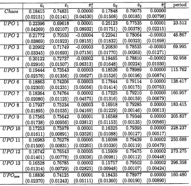
First,

we

show Table 1, where the statistical data of the chaotic solution

and the unstable periodic solutions

are

listed. In the table, the data of

$UPO_{ave}$ is calculated

as

below:

$\overline{x}_{UPO_{av\mathrm{e}}}=\frac{\Sigma_{k=1}^{13}\overline{x}_{UPOk}}{13}$. (9)

The statistical data of $UPO7$ _and $UPO_{ave}$ resemble that of Chaos well.

It implies that behaviors

on

unstable periodic orbits would be connected

$13\mathrm{S}\mathrm{e}\mathrm{e}$

Kazantsev(1998).

$14\mathrm{W}\mathrm{e}$definethe unstable

periodic orbit with$n$whirlsas$UPOn$.

$16\mathrm{S}\mathrm{t}\mathrm{a}\mathrm{t}\mathrm{i}\mathrm{s}\mathrm{t}\mathrm{i}\mathrm{c}\mathrm{a}\mathrm{l}$

datapresentedinthenext section willanswerthis question.

with the chaotic fluctuation

over

along time. Now,

we

will discuss this

point further.

Table 1: Mean values of variables ofChaos and UPOs

The figures inparenthesesarethevariances correspondingto economic variablesof the system.

To

see

differences not appearing in low order statistics(mean and

vari-ance), we illustrate histograms. Fig.4

upper

left shows three histograms

calculated from the movements of the labor share rate in country 1. The

first

one

is depicted through the long time movement enough to represent

the statistics ofchaos, the second is $UPO7$, and the last

one

is $UPO_{ave}$

.

We find the histogram of $UPO_{ave}$ approximates best that of chaos in the

case

of variable $u_{1}$

.

In practice, regarding other variables,

we

obtain the

similar results.(See other histograms.) We

can

consider that the chaotic

orbit will pass many times by every unstable periodic orbits in the chaotic

attractor, therefore the statistics ofthe chaotic solution and the unstable

periodic solutions

are

very similar.

Fig. 4: Histograms ofChaos, $UPO7$, and $UPO_{ave}$

Another evidence

we

present to point out the similarity is Fig.5. The

Lyapunov dimension calculated for

our

parameter setting

are

plotted in

this figure. The Lyapunov dimensionofthe chaotic attractor is denoted by

the horizontal dashed line, and that ofeach unstable periodic orbit found

in the attractor corresponds to individual dot in the figure. All dots,

except for $UPO1$,

are

_depicted

near

the line. Particularly the unstable

periodic orbits with 9, 10 and 11 whirls have the similar properties to the

chaotic attractor in terms of the Lyapunov dimension. On the otherhand,

it

can

be considered the chaotic orbit seldom passes close the shortest

periodic orbit, and it

means

that the economicregime corresponding $UPO$

$1$ is seldom

seen

in the chaotic fluctuation

.16

$16\mathrm{T}\mathrm{h}\mathrm{e}$

relation between theperiodofthe unstableperiodicorbit andthesimilarityof the orbit to the chaotic attractorismeaningful, though it isnotdiscussed anymorein thispaper.

6

$\mathrm{C}\cap \mathrm{a}\mathrm{o}\mathrm{s}\cup \mathrm{P}\circ$ 4 5 $.\dot{rightarrow}3\not\geqq\Leftarrow\infty 4\simeq\Leftarrow$ $\varpi \mathrm{a}_{\mathrm{z}}\cong>$ $—–*——-\neq---*---\pm---\neq---*---\star---arrow---\wedge---*$ s— $-\lrcorner>$ $\cup \mathrm{P}\mathrm{O}1\mathrm{Q}$

$\cup \mathrm{P}\propto$ $\mathrm{U}\mathrm{P}\mathrm{O}3$ $\mathrm{U}\mathrm{P}\mathrm{O}4$ $\cup \mathrm{P}\mathrm{O}6$ $\mathrm{U}\mathrm{P}\mathrm{O}6$ $\cup \mathrm{P}\mathrm{O}7$ $\cup-\mathrm{O}8$ $\mathrm{U}\mathrm{P}\mathrm{O}9$ UPOI$0$ _LiPOII $\mathrm{U}\mathrm{P}\mathrm{O}12$ $\cup \mathrm{P}\mathrm{O}13$

Fig. 5: Lyapunov dimension ofChaosand UPOs

From the physical point of view, it is well known there

are some

stable

dimensions

as

regards unstable periodic orbits though they have

instabil-ity. In fact, the stable directions

are

considerably abundant in

our

system.

These must be the

reasons

why typical dynamics of chaotic solutions exist

analogous to the unstable periodic orbits in this study. Thus

our

model

displays the various economic regirnes related to unstable periodic orbits.

Now,

we

go

on

with

our

discussion from the proposition that

unsta-ble periodic orbits

concern

the economic regimes experienced

on

the long

term growth trajectory. To be argued

are

the effects of the variation of

each parameter

on

the growth path where the economy should go. For

ex-ample, the increase in public spending mayimprove the domestic business

cycles for the time being. Ifwe examine the variation and deformation of

unstable periodic orbits by the change in apolicy parameter,

we

can

un-derstand the effect

on

the growth path

more

clearly. Because the unstable

periodicorbits have quite simple structure although they

are

qualitatively

and quantitatively similar to the chaotic orbits. Concerning this point,

we will discuss in detail in the next paper.

5Conclusions

We have given agrowth cycle system with international trade and shown

some

unstable periodic solutions found numerically in the chaotic

attrac-tor. It is cleared that they explain atypical long

run

dynamics consisting

of asequence of short

run

trade cycles and have the features

correspond-ing to the long

run

movements classified as the economic regimes on the

chaotic growth path. In addition,

we

have shown that the statistical

properties of the chaotic fluctuation in the model

are

approximated to

aconsiderable extent by those ofthe unstable periodic orbits. It implies

unstable periodic solutions

can

be the keywords to understand the chaotic

dynamics. From the above results, we ernphasize the importance and

use-fulness of unstable periodic solutions embedded in the chaotic attractor

as objects of studies of chaotic behavior. Above all, this point is

impor-tant when we discuss the impacts of the economic policy in the chaotic

situation. References

[1] Desai, M.

1973.

Growth Cycles and Inflation in aModel of the Class

Struggle, Joumal

_of

Economic Theory, Vo1.6, pp.527-545.

[2] Goodwin, R. M. 1967.

AGrowth

Cycle, in Socialism, Capitalism, and

Economic Growth, Essays Presented to Maurice Dobb, C. H. Feinstein

(ed.), Cambridge University Press, Cambridge, pp.54-58.

[3] Goodwin, R. M. 1990. Chaotic Economic Dynamics, Oxford

Univer-sity Press,

Oxford.

[4] Ishiyama, K. and Saiki, Y. 2003. Unstable Periodic Solutions

Embed-ded in aChaotic Economic Dynamics, preprint.

[5] Kato, S. and Yamada, M. 2002. Unstable Periodic Solutions

Embed-ded in aShell Model Turbulence, $prep_{7}\dot{\tau}nt$

.

[6] Kawahara, G. and Kida, S. 2001. Periodic Motion Embedded inPlane

Couette Turbulence: Regeneration Cycle and Burst, Jorrrnal

_of

Fluid

Mechanics, Vo1.449, pp.291-300.

[7] Kazantsev, E. 1998. Unstable Periodic Orbits and Attractor of the

Barotropic

Ocean

Model, Nonlinear Processes in Geophysics, Vo1.5,

$\mathrm{p}\mathrm{p}.193- 208$

.

[8] Skott, P.

1989.

Effective Demand, Class Struggle, and Cyclical

Growth, International Economic Review, Vo1.30, NO.1, pp.231-247.

[9] Takamasu, A.

1995.

On the Effectiveness of Fiscal Policy in the

Goodwin’s Growth Cycle Model, in Proceedings

_of

the International

Conference

on

Dynamical Systems and Chaos, N. Aoki, K. Shiraiwa,

and Y. Takahashi (eds.), World Scientific Publishing, Singapore,

Vol.l, pp.433-436.

[10] Wolfstetter, E.

1982.

Fiscal Policy and the Classical Growth

Cy-cle,

_Zeitschrift

_f\"ur

_{National\"okonomie/Journal}

_of

Economics, Vo1.42,

N0.4, pp.375-393.

[11] Yoshida, H. and Asada, T. 2001. Dynamic Analysis of Policy Lag in

aKeynes-Goodwin Model: Stability, Instability, Cycles and Chaos,

preprint.

[12] Zoldi, S. M. and Greenside, H. S. 1998. Spatially Localized

Unsta-ble Periodic Orbits of aHigh-Dimensional Chaotic System, Physical

Revieev E, Vo1.57, N0.3, pp.2511-2514.