Teleportation of position and momentum of a quantum state in terms of a correlation function of the Gaussian type : A time-dependent model (Algebraic Systems, Formal Languages and Conventional and Unconventional Computation Theory)

(1)

177

Teleportation of position andmomentumof

a

quantumstateintermsof

a

correlationfunctionof theGaussian type:A time-dependentmodel

K.Saito and$\mathrm{F}.\mathrm{M}$

.

Toyama

DepartmentofInformation andCommunicationSciences,Kyoto SangyoUniversity, Kyoto

603-8555, Japan

We present atime-dependent model that explicitly describes, in coordinate space,

teleportation of a quantum state of position and momentum. Teleportation of an

unknownquantum state is performed by meansof quantumentanglement and classical

communication. We assumethat the quantum entanglement is expressed in termsofa

correlation function of the Gaussian type that is reduced to the EPR state in the

6-function limit. We analyze anoptimal situationin whichahigh degreeofteleportation

fidelity and a large teleportation probability areachieved. We also discuss asituation

where thetime delaydue to theclassicalcommunicationcannot be ignored.

1.Introduction

Bennett et al. [1] _proposed

_a

_{protocol of}quantum teleportation of

an

unknown spin-1/2 state

in terms of

a

maximally entangled spin state shared by Alice (sender) and Bob (receiver).

Vaidman [2] _{analyzed teleportation of}

an

_{unknown quantum state of} _continuous _{variables such}

as

position and momentum in terms of the EPR (Einstein, Podlsky and Rosen) state 13] that

represents perfect correlations in both variables. Braunstein and Kimble [4] extended Vaidman’s

analysis to incorporate incomplete correlations in both variables and inefficiencies in the

measurement

process.

Theyalso provided

a

scheme for realistic implementationofteleportation

of continuous variables, using quadrature amplitudes of the electromagnetic field. Furusawa et

al.[5]examinedexperimentally such

a

scheme.

The protocol of quantum teleportation consists of three ingredients, i.e.,

a

quantum

entangled statethatisshared by Alice and Bob,

an

entangle-measurement byAlice and

a

unitary transformation of

a

state generated at Bob’s site. In order toperformthe unitary transformation

Bobhas to know the results of the measurement done byAlice.Therefore,Alice informs Bobof

the results of her measurement by classical communication. The classical communication is

an

indispensable part of the protocol. However, Bob cannot always restore the

same

state

as

the input state by the unitary transformation. This inefficiency ofthe teleportation is mainly due to the incompleteness ofthe entanglement and the measurement process. Here,

we

point out that

there exists another factor that

causes

inefficiency in the teleportation. A time delay due to

classical communication allows the post-measurement state generated at Bob’s site to develop

over

time. In

a

situation where the time-evolution of the post-measurement state befo the

unitary transformation is not negligible,

we

have totake account of such time-evolution ofthe

post-measurementstate.

The

purpose

of the present work is to investigate such inefficiencies in quantum

teleportation of continuous variables. For this

purpose

we

present

a

time-dependent model that explicitly describes, in coordinate space, the

process

of the teleportation of momentum and position.

(2)

178

2.Atime-dependentmodel

We consider three particles that

we

designate

as

12and 3, respectively. Alice and Bob share

an

entangled state $|\mathrm{v}_{23}^{\mathrm{Z}}\mathrm{o}$

))

ofparticles 2and3.To teleport

an

input state $\wedge|\psi_{1}$$(t)\rangle$ of particle 1 to

Bob, Alice does the measurements of two commutative observables $X_{12}=\hat{X},$$+\hat{x}_{\underline{2}}$ and

$\hat{P}_{1_{-}},\cong$

$\hat{p}_{1}$-$\hat{p}_{-}$, of particles 1 and 2, where $\hat{X}_{j}$ and $\hat{p}_{i}$ $(i =1,2)$

are

respectively the position and

momentumoperatorsofeach particle. When Alice doesthe measurementsof $X_{1_{-}}$, and $P_{12}$,

a

state

$|\psi_{3}(t)\rangle$ of particle 3 is generated at Bob’s site. Except for

a

special case, the generated state

$|\psi_{3}\mathrm{O})\rangle$is differentfrom the input state $|\mathrm{p}_{1}(t)\rangle$

.

Inordertocompletetheteleportation, Bob hasto

transform $|\psi_{3}(t))$ to $|\psi_{1}(t)\rangle$

.

The transformation is realized by

a

unitary operator that is

determined with the results of the measurements of $\hat{X}_{12}$ and

$P_{12}$, Alice informs Bob of the

results of her measurement by classical communication

so

that Bob

can

perform the unitary

transformation.

Fortheunknowninputstate $|\psi_{1}(t)\rangle$,whichAlice wants to teleportto Bob,

we

take it

as

$|\psi 1$$(t)\rangle-N_{1m}[|\phi^{+}(t)\}+|\phi_{1}^{-}(t)\rangle]$, (2.1)

where $|\mathrm{c}(\mathrm{r}))$

are

normalized tounity and $N_{1n}$, istherenormalizationfactor. For $|\mathrm{c}(t))$

we

take

themincoordinaterepresentation

as

$\phi^{\mathrm{f}}(x_{1},t)$\approx$\{x_{1}|0^{\mathrm{f}}$$(f)\rangle^{N}-\sqrt{1+\frac{\iota_{i\hslash t}}{m\sigma_{1}^{2}}}^{\exp\{-\frac{(X_{1}-X_{0}^{\mathrm{f}}-\frac{\hslash K^{\mathrm{f}}}{m}\mathfrak{l})^{2}}{2\sigma_{1}^{2}(1+\frac{i\hslash t}{m\sigma_{1}^{2}})}+i[K^{*}(x_{1}-x_{0}^{\mathrm{r}})-\frac{\hslash K^{*2}}{2,n}t]\},(2.2)}$

where $N_{1}$ -$(M_{1}^{-}’)^{-1l4}$ is the normalization factor, $m$ is the

mass

of particle 1, $\sigma_{1}$ and

$K^{\mathrm{f}}$

are

respectively the width and

wave

numbers of the

wave

packets $\phi^{*}(x_{1},r)$

.

The

wave

packets

$\mathrm{A}$’(x1’$r$)

are

solutions of the free Schr\"odinger equation. In numerical illustrations

we

will take

$r$

as

$K^{*}\sim-K^{-}$

.

For such

a

choice of $\kappa$, the input state $|\psi_{1}(t))$ is

a

tw0-mode state. For Eq.

(2.2)therenormalization factor $N_{1n}$, is given

as

$N_{1rn}-\{2[$$1+ \exp(-\frac{(x_{0}^{*}-x_{0})^{2}}{4\sigma_{1}^{2}}-\frac{\sigma_{1}^{2}(K^{+}-K^{-})^{2}}{4}]\cos(\frac{(K^{+}-K^{-})(x_{0}^{-}-x_{0}^{+})}{2})]\}^{-\frac{1}{2}}$ (2.3)

TheWigner distribution [6]_{of the}inputstateisexpressed

as

$W_{in}(_{X_{1’ h}},t)- \frac{1}{2M\iota}\int_{-\#}^{\infty}$\Phi $\exp(i\frac{p_{1}y}{\hslash})\{x_{1}+\frac{y}{2}|\hat{\hslash}(t)|x_{1}-\frac{y}{2}\}$, (2.4)

where $\hat{\rho}_{\mathrm{I}}(t)$ is the density matrix of the input state, i.e., $\mathrm{j}(t)$=$|\mathrm{V}_{1}(\mathrm{t}))\langle\psi_{1}(\mathrm{r}1$ The Wigner distribution(2.4)is useful in seeing thequantumcoherence in$|\mathrm{p}_{1}(t)\rangle$

.

Next,

we

consider the measurement sate for Alice. We suppose that Alice does her

(3)

17S

-in $(\partial/\partial x_{1}-\partial/\acute{\mathrm{d}}x_{2})$ at $t=0$. In

our

model

we

representthemeasurement state at $t=0$

as

$\chi_{a,b}(x_{1},x_{2})\Xi$$\langle x_{1}x2|\chi_{a}$

,$b)$

$\approx$$N_{12} \exp[-\frac{1}{2\mathit{0}_{12}^{2}}(x_{1}+x_{2}-a)^{2}-\frac{1}{2\sigma_{12r}^{2}}(x_{1}-x_{2})^{2}$$+$ $i(k_{1}x_{1}+p_{\overline{Z}}x_{2}.)]$,

(2.5)

where $\sigma_{12}$ and $\sigma_{1u}$

are

respectively the distribution parameters of the center-0f-mass and

relative motions, $k_{1}$ and

4 are

the averaged

wave

numbers of particles 1 and 2, $b\sim$ $k_{1}-k_{2}$ and

$N_{12}$-$(2\mathit{1} \pi\sigma_{12}\mathit{0}_{12r})^{\mathrm{I}2}$ isthenormalizationfactor. Interms of Eq.(2.5) theexpectation values of $\hat{X}$

,,

and $\hat{P}_{12}$

are

given

as

$\langle\chi_{a,b}|X_{12} |\chi_{a.b}\rangle$_$-a$ and $\langle\chi_{a.b}|\hat{P}_{12}|\chi_{a.b}\rangle$

.

$\hslash(k_{1}-k_{2})i\hslash b$

.

(2.6)

For {$\sigma_{12}arrow$ very small, $\sigma_{1-},$$arrow$ very large}, two equations of Eq. (2.6) approach the following approximate eigenvalue equations, i.e., $X\wedge 12|Xa.b$

)

$\sim$$a|\chi_{a,b}\rangle$ and $\hat{P}$

1

$2|\chi_{a.b}\rangle$$\sim\hslash b|\chi_{a,b}\rangle$

.

Here, the

perfect limit of {$\sigma_{2},arrow 0$, $y_{12r}arrow\infty\rangle$ is not physical in the

sense

that Eq. (2.5) approaches

a

measurement state of the $\delta$-function type with

an

infinitely small normalization factor

$2(\sigma_{12}/\sigma_{12r})^{1/2}$ inthelimit.

Here let

us

considerthe correlationstate $|\psi_{\mathfrak{B}}(t)\rangle$ between particles 2and 3 which is shared

by Alice andBob. We assumedthat Alice does her measurements at $t=0$. Therefore, in factwe

need $|\psi_{23}(t. 0)\rangle$

.

Forthecorrelation at $t$

=0

we assume

theGaussiantype, $\psi_{23}$$(x_{2},x_{3},t - 0)$\approx$\langle$x_$2^{X}3|$$\mathrm{j}_{23}(t-0)\rangle$

$\sim$$N_{23} \exp[-\frac{(x_{2}+x_{3})^{2}}{2\mathit{0}_{B}^{2}},-\frac{(x_{2}-x_{3})^{2}}{2\mathit{0}_{\mathfrak{B}r}^{2}}+ik_{23}(x_{2}+x_{3})+ik_{23r}(x_{2}-x_{3})]$ ,

(2.7)

where $\sigma_{-3}$, and $\sigma_{s}$

,, are

thedistributionparameters of thecenter-0f-massandrelativemotionsof

thetwoparticles,

₄

and $h_{-3}$,

are

the

wave

numbersfor thecenter-0f-massand relativemotions

and $N_{23}$-$(2/\pi \mathit{0}_{23}\sigma_{23r})^{1l2}$ is the normalization factor. If $\mathrm{z}_{s},=\mathit{0}_{s},$,, Eq. (2.7) has

no

correlation between $x_{-}$, and $X_{3}$

.

Infact,

we

examine

cases

where $\sigma_{-3}$, is very smalland $\sigma_{\underline{\mathrm{o}}_{3}}$, is very large.

Further, Eq. (2.7) has

no

correlationfor the center-0f-mass and relative coordinates $(x_{-},+x_{3})f2$

and $x_{2}-x_{3}$

.

When $h_{Sr}\# 0$, Eq. (2.7) is neither symmetric

nor

anti-symmetric fortheexchange

of particles 2 and 3. Therefore, in numerical illustrations

we

will take $h_{\lrcorner}$, to be 0. The

expectation valuesoftwocommutativeobservables $\hat{X}_{\lrcorner},=\hat{X}_{-},+i_{3}$ and $\hat{P}_{\mathfrak{B}}\mathrm{r}\hat{p}:-\hat{p}_{3}$intermsof Eq.

(2.7)

are

$\langle\psi_{\mathfrak{B}}(t-0)|\hat{X}_{\mathfrak{B}}|/\mathfrak{B}(t=0)\rangle$-0 and $\langle \mathrm{i}\mathrm{j})_{23}(t - 0)|P2 |\psi_{\mathfrak{B}}(t - 0)\rangle$ _-$2f_{1}k_{23r}$

.

(2.8)

Inthelimit of {$\sigma_{3}\underline,arrow$ very small, $\sigma_{3}\underline,,$$arrow$ very large}, Eq.(2.8)

can

be regarded

as

approximate

eigenvalue equations $\hat{X}_{\mathfrak{B}}|l$_{$\mathfrak{B}/-0|$}

$J$$23\rangle$ and $\hat{P}_{-3},|$$/23\rangle$ $\sim 2\hslash k_{23r}|\psi_{\mathfrak{B}}\rangle$ Here, the perfect limit of

$\{\sigma_{3\sim},arrow 0, \sigma_{-3},, arrow\infty\}$ isnot physical because Eq. (2.8) approaches

a

correlation function of the

$\delta$-functiontype withtheinfinitelysmallnormalizationfactor $2(\sigma_{23}/\sigma_{23r})^{1l2}$ in thelimit

When Alice doesthe measurements of $\hat{X}_{1_{-}}$, and $\mathrm{E}_{\underline{2}}$ at $t-0$,

a

state _{$|\psi 7_{3}(t-0))$} of particle3is

(4)

180

We call the generated state the post-measurement state hereafter. We describe the measurement

process

as

$\langle\chi_{a,b}| j_{1}(t\approx 0)\otimes 7_{\mathfrak{B}}(t\Leftarrow 0)\rangle|_{I2}=\sigma$$|\psi_{3}(t=0)\rangle$, (2.9)

where ₉ is the probability amplitude for generating $|$$p_{3}(e=0)\rangle$

.

The post-measurement state

$|\mathrm{t}/3(t = 0)\rangle$consistsof twocomponents, i.e.,

$|$$/3(t-0)\rangle-N_{3m}[|\phi’(t=0)\rangle+|\phi_{3}^{-}(t-0)\rangle]$, (2.10)

where $N_{3n}$, isthenormalizationfactor. By usingEqs. (2.1),(2.5) and(2.7) the component states

$|\phi$

;

$(t$-0$)$

)

inEq.(2.10)

can

explicitly begiven incoordinate

space as

$\phi_{3}^{\mathrm{f}}(x_{3},t = 0)$$\cdot\{x_{3}$$|\phi_{3}^{\mathrm{f}}(t-0)\rangle$

$- \exp[L_{0}^{\mathrm{f}}+\frac{L_{1}^{\mathrm{r}2}}{L_{2}}+i(\frac{M_{1}^{\mathrm{f}}L_{1}^{*}}{L_{2}}+M_{0}^{*})]\exp[-L_{2}(x_{3}-\frac{L_{1}^{*}}{L_{2}})^{2}+iM_{1}^{*}(x_{3}-\frac{L_{1}^{\mathrm{f}}}{L_{2}})]$,

(2.11)

where $\mathit{1}_{\triangleleft}^{\mathrm{f}}$ _\approx$I^{*2}lH+$$(Aa +Cx_{0}^{*})^{2}/F-k_{a}^{*2}\mathit{1}F$ $-(k_{b}-k_{a}^{\mathrm{f}}G/F)^{2}\mathit{1}4H-Aa^{2}-Cx_{0}^{*2}$,$l_{4}^{\mathrm{f}}$ -$21^{*}J\mathit{1}H$,

$h-D\dagger E-J^{2}\mathit{1}H$_,$M_{0}^{*}=-K" x_{0}^{\mathrm{f}}+ka*$$(Aa-Cx_{0}^{*})\mathit{1}F-I^{1}$($k_{b}-k_{a}^{*}G$fF)lH and$M_{1}^{*}-J(k_{c}-k_{b}$ $+k:GIFi\mathit{7}H$ with$A$ $-1\mathit{1}2\sigma_{12}^{2}$,$B\cdot 1/2\sigma_{12r}^{2}$, C-ll$2\sigma_{1}^{2}$,$D=1\mathit{1}2\sigma_{\mathfrak{B}}^{2}$,$E=1\mathit{1}2\sigma_{\mathfrak{B}r}^{2}$, $F-A+B+C$

,

$G-A-B$, $H-A+B+D+E-G2$1$F$, $I^{\mathrm{f}}-G(Aa+Cx_{0}^{\mathrm{f}})$IF-Aa, J.$D-E$,$h_{l}^{*}$-$K^{\mathrm{f}}-k_{1}$,$k_{b}-k_{\mathfrak{B}}$

$+k_{23},$ $-k_{2}$and $k_{c}’-k_{\mathfrak{B}}$

-kl3r.

For $\mathrm{A}^{\mathrm{f}}$of Eq.(2.11) _{$N_{3n}$}, isgiven

as

$N_{3m}-\{\sqrt{\frac{\pi}{2L_{2}}}[$_$\exp$

(2

$(L_{0}^{+}+ \frac{L_{1}^{*2}}{L_{2}}))+\exp($2$(L_{0}^{-}+ \frac{L_{1}^{-2}}{L_{2}}))$

$+2\exp$

(

$\mathit{1}_{0}^{+}+I_{0}+\frac{1}{2L_{2}}(L_{1}^{+}+4)^{2}-\frac{1}{8L_{2}}(M_{1}^{+}- \mathrm{A}\mathrm{t}_{1}^{-})2$

)

$\cos(\frac{(M_{1}^{+}-M_{1}^{-})(L_{1}^{+}+L_{1}^{-})}{2L_{2}}+M_{0}^{+}-M_{0}^{-})]\}^{-\frac{1}{2}}$

(2. 12) By usingEqs. (2.1), (2.5) and(2.7),from Eqs.(2.9) and(2.10)thegeneration probability

can

be

obtained

as

$| \sigma|^{2}-(\frac{\pi N_{1}N_{12}N_{23}N_{1m}}{\sqrt{FH}N_{3m}-})^{2}$ (2.10)

The $|\sigma|^{2}$ is

a

functionofpmmeters

7), $\mathrm{z}_{\sim},$,,$\sigma_{1x}$, , $\mathrm{v}_{\sim},3$

’ $\sigma_{\mathfrak{B}}$,, K.

$x_{0}^{*}$, _$a$, $k_{1}$,k-, $h_{3}$ and $h_{s}$,.The

post-measurement state $|$_{$p_{3}(t$}-0$)$

}

of Eq. (2.10) is different from the input state $|$

vq

$(t$-0$)$

},

exceptfor

a

special

case

wherethe correlation between particles 2 and 3 is the 6-function type

and the results of the measurement of $\hat{X}_{12}$ and $\hat{P}$

g2 are both0. In order to complete the

teleportation Bob has to transform $|\mathrm{w}_{3}(t-0)\rangle$ into

$|\mathrm{w}\mathrm{r}^{1}$$(t))$ by

a

unitary transformation

$\hat{U}(a,b)$

(5)

181

her measurements $a$ and $\hslash b$ to Bob using classical communication. This classical

communication

causes a

time delay. In

a

situation where

we

cannot ignore such

a

time delay

we

have to take into account the time-evolution of the post-measurement state. If

we

suppose that

the post-measurement state evolves in free

space,

we

can

write down the time-evolution of the

post-measurementstate ofEq.(2.10)analytically

as

$|$

$/3$$(t)\rangle-N_{3rn}[|\phi$

;

$(t)\rangle+|\phi_{3}^{-}(t)\rangle]$ . (2.14)

where

$\phi_{3}^{*}(x_{3},t)\cdot\langle x_{3}|\phi_{3}^{*}(t)\rangle-\sqrt{1+i\frac{12L_{2}\hslash t}{m}}\exp$

$[L_{0}^{*}+ \frac{L_{1}^{*2}}{L_{2}}+i(\frac{M_{1}^{\mathrm{f}}L_{1}^{*}}{L_{2}}+M_{0}^{*})]$

$\mathrm{x}$$\exp\{-\frac{L_{2}(x_{3}-\frac{l_{1}^{*}}{L_{2}}-v_{0}^{*}t)^{2}}{1+i\frac{2L_{2}\hslash t}{m}}+i[M_{1}^{*}(x_{3}-\frac{L_{1}^{*}}{L_{2}})-\omega_{0}^{*}t]\}$

.

(2.15)

(2.16) InEq.(2.15),$v_{0}^{\mathrm{A}}11\hslash M_{1}^{*}/m$ and $a\iota^{*}=$$\hslash M_{1}^{*2}l\mathrm{h}\iota$

.

The

wave

functions(2.15)

are

solutions ofthe

freeSchr\"odingerequation.

Theunitarytransformation $\hat{U}(a,b)$ is expressed incoordinate space

as

$\hat{U}_{x}(a,b,x_{3})$

.

$\langle$

$x_{3}$

l\^U(a,b)l

$x_{3}$$\rangle$_$-$_$\exp$$\{i[(b+2k_{\mathfrak{B}r})\hat{x}_{3}-\frac{a\hat{p}_{3}}{\hslash}]\}\exp(iak_{1})$,

where $\hat{p}_{3}$- $-ih$$\partial/\partial x_{3}$

.

The constantphasefactor $\exp(iak_{1})$ in Eq. (2.16)arises inthe 6-functi0n

limit of $|\mathrm{v}_{23}(t)\rangle$ and $|x_{a,b}\rangle$$[2]$

.

TheWignerdistribution of the post-measurement state $|\mathrm{y}\mathrm{z}_{3}$$(t))$ is expressed

as

$W_{om}(x_{3\prime}p_{3},t)- \frac{1}{2\mathrm{f}\mathrm{f}\mathrm{i}}\int_{-\infty}^{\infty}dy\exp(i\frac{p_{3}y}{\hslash})\langle x_{3}+\frac{y}{2}|\hat{/}3(t)|x_{3}-5\rangle$, (2.17)

where $\hat{\rho}_{3}(t)$-$|\psi_{3}(t)\mu\psi_{3}(t)|$

.

Forthe Wignerdistribution $W_{ou},(x_{3},p_{3}, t)$ ofEq.(2.17),theunitary

transformation $U$(a,b) of Eq. (2.16) is just the shift operation $\{$_{$X_{3}arrow$}

$x_{3}-a$, $p_{3}arrow p_{3}-h(b+2k_{\lrcorner r},)\}$, namely $W_{ou\ell}^{\prime el}(x_{3},p_{3},t)-W_{ou}(x_{3}-a,p_{3}-\mathrm{h}(b+2k_{23r}),$$t)$

.

The fidelity $F(t)$

of the teleportation is defined

as

$F(t)-\langle \mathrm{V}\mathrm{t}(t-0)|\hat{p}_{ou}^{\prime el},(t)|\mathfrak{R}(t-0)\rangle$, (2.18)

(6)

182

3.Numerical illustrations

In numerical illustrations

we

assume

that $m$ is the electron

mass

and

use

atomic units. Then $mrightarrow 1$, $\hslash-1$ and _$c$-137. The unit length is the Bohr radius. Figure 1 shows the Wigner

distribution $W_{in}$$(x_{1},p_{1}, t - 0)$ of the input state $|\mathrm{y}_{1}(t-0)\rangle$ ofEq. (2.1). For the parameters of the

input state

we

took them to be $\mathrm{v}_{1}-5$, $x_{0}^{+}\sim-5$, $x_{0}^{-}\sim-7$ and $K^{\underline{\mathrm{r}}}$

.t0.5. The distribution

$W_{in}$$(x_{1},p_{1}, t. 0)$ has

an

oscillation with negative distribution between the two positive

distributions around$p_{1}\sim \mathrm{f}$5. This represents quantum coherence due to the terms

$|\mathrm{A}^{+}(t-0))\langle\phi^{-}(t. 0)|$ and $|4-(t-0)\mathrm{Q}’(t-0)|$in $\hat{\rho}_{1}(t-0)$

.

(a) _(b)

First,

we

examine the generation probability $|\sigma|$’ of the state $|\psi_{3}(t-0)\}$

.

Figure 2 exhibits

the behavior of $|\sigma|$’ for the parameters $\sigma_{12}$ and $\sigma_{23}$ that represent distributions of the center-of-mass motions in the measurementand the correlation state. Figure $2\mathrm{a}$ is the

case

where the

results ofmeasurementby Alice

are

assumed to be $a-hb$.0. Thegeneration probability $|\sigma|$

’

is

very

small

as

a

whole. For smaller $\sigma_{1_{-}r}$

.

and $\sigma_{\mathfrak{B}}$,

’ $|\sigma|$

’

becomes larger. However, the smaller $\mathrm{q}_{2r}$ and $\sigma_{23r}$ are,the smaller the fidelitybecomes.Therefore, inFig. 2

we

fixed theparameters

$o_{1x}$, and $\sigma_{\lrcorner r}$, tobe

10’

toget

a

high fidelity. An interesting feature of $|\sigma|$ ’

(7)

183

maximum in a small $(\mathit{0}_{12},\mathit{0}_{\mathfrak{B}})$ region. The position of the local maximum is around $(\mathrm{a}12, \mathrm{v}_{\mathfrak{B}})$ $-(1.65,1.65)$ for the

case

of $a\sim\hslash b$-0. Figure $2\mathrm{b}$illustrates the shift of the position of

the maximumfor $b$

.

As the shiftof the local maximum isnotsensitiveto $a$,

we

fixed itto be 2

in the illustration.The local maximum shifts to

a

largerregion of $\sigma_{1j}$ and $\sigma_{\lrcorner}$, for larger $b$

.

For

$b\mathrm{z}$$0.2$ the maximum in the small $(\sigma_{12},\mathit{0}_{23})$ region disappears and around $b-0.8$ it reappears.

Actually thereexists

a

big bump in

a

very large $(\sigma_{12},\sigma_{23})$ region. For 0.2\leq bs0.8,the bump in

such

a

large $(0_{12},\circ_{\mathfrak{B}})$ region masks the local maximum inthe small $(\sigma_{12},\sigma_{\mathfrak{B}})$ region.

(b) _{$W_{m}^{\nu l}(x_{3}.p_{3},’-4)$}

5

.1

-

—.—

$P_{3}$ $x_{3}$

Fig. 3(a) The Wigner distribution $W_{o1P}’’’(x_{3},p_{3},t-0)$ of the output state $|?\mathrm{i}’ \mathrm{O}-0$

))

$-$

$\hat{U}(a$_-2,_{$b-0.11\psi_{3}(t$}_-0

$)$

}.

The fidelity is $F(t - 0)-$0.999. (b) The Wigner distribution

$W_{nu}’’,(x_{3},p_{3},t-4)$ of the output state _$|1/3’$”₍$t$.s4)$)-\ddot{U}(a-2. b- 0.1)$$|\mathrm{V}_{3}$$(t-4)\rangle$

.

The Fidelity is

$F(t-4)-$0.885. The results of the measurement by Alice are assumed to be

$a$-2, $b$-0.1 _{$(k_{1}- 0.1, k_{2}-0)$}

.

The parameters of $|\chi_{a.b}\rangle$ and $|\psi_{23}$) are $h_{-3}-k_{-3}$,

$,$ -0,

$\sigma_{J},,-\sigma_{\lrcorner},-r10^{3}$ and $0_{1_{-}},$$-\sigma_{\lrcorner}$, $-10^{-3}$

.

Theunitsareatomic units.

Figure $3\mathrm{a}$ shows the Wigner distribution _{$W_{ow}’(x_{3},p_{3},t-0)$} of the output state

$|{}^{\mathrm{t}}\mathrm{P};^{1}\mathrm{O}-0$ ).

where $a-2$ _and

_b-O.11

$h$$-0.1$, $k_{2}$ \sim 0); $b\sim 0.1$ corresponds to 1/1370of $c$

.

Otherparameters

of $|\psi_{\mathfrak{B}}$

)

and $|\chi_{a.b}\rangle$

are

takentobe _{$h_{s}-k_{S}$},

$,$ -0, $\sigma_{1x}$, $.a$$\sigma_{\lrcorner}$, ’ @E $10^{3}$ and $\sigma_{1_{\sim}}$,-$\sigma_{-3}$, -$10^{-3}$

.

Note that

$\sigma_{12r}$ and $\sigma_{23}$,

are

very

largeand $0_{12}$ and $\sigma_{\mathfrak{B}}$

are

very

small.Thischoice of the parameters $\sigma_{1u}$,

a23 $0_{12}$ and $\sigma_{23}$ gives

a

situation close to the

$\delta$-function limit of the measurement and

correlationstates.As

seen

inthefigure $W_{au}’(x_{3},p_{3},t-0)$ isalmost the

same as

Wln$( \mathrm{r}_{1},p_{1}, t- 0)$ of

the input state. The fidelity is

very

high in this case, i.e.,$F(t$ -0$)$-0.999,

as

expected. The teleportationin thissituation

seems

quite successful. However,

as seen

in Fig. $2\mathrm{b}$the generation probability $|\sigma|^{-}$

’

is verysmall inthis

case.

Thus,although

we

can

achieve teleportation with high

fidelity by supposing

a

situation close to the $\delta$-function limit of the measurement and

(8)

184

Figure $3\mathrm{b}$ exhibits $W_{\mathit{0}l\ell}^{\mathfrak{l}rl},(x_{3},p_{3},t-4)$, which illustrates the time-evolution of the

post-measurement state $|’ \mathit{3}‘ el$$(t-4)\rangle$. As

a

typical

case we

have shown the

case

of

$\mathrm{f}$-4

$(.9.676 \mathrm{x}10^{-17}\mathrm{s})$

.

The difference between $W_{ou1}’(x_{3},p_{3},t-4)$ and $W_{o\downarrow u}^{rl}’(x_{3},p_{3},t-0)$ is

appreciable. The fidelity at r-4 is $F(t$-4$)$-0.885, which is much reduced from

$F(t$ -$0\rangle$_$-$0.999. Thus, in the present analysis, the effect of the time-evolution of the

post-measurementstate before theunitarytransformation becomesappreciable around $t-4$

.

$W_{ou}^{\kappa l}(x_{3},p_{3\prime}’-0)$

$p_{3}$ $\mathrm{K}_{3}$

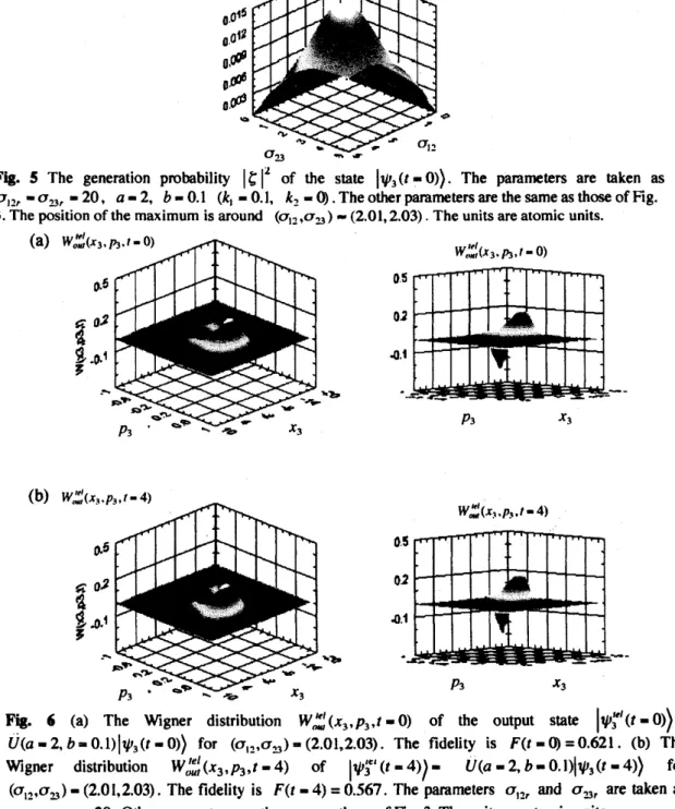
Next, we consider a situation that corresponds to the local maximum of $|\sigma|$’ in the small

$(\sigma_{12}, \sigma_{\mathfrak{B}})$ region.The $|$

$9$$|$ ’

has the local maximum around $(0_{12}, \sigma_{2})$-(1J7, 1.87) for $a-2$ and

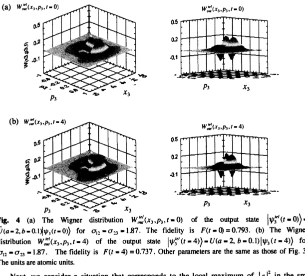
-0.1 $(k -0.1, h_{\sim}-0)$_(see Fig. $2\mathrm{b}$). Figures$4\mathrm{a}$and$4\mathrm{b}$show the outputs _{$W_{w}’,(x_{3},p_{3},t-0)$} and

$W_{o\alpha\iota}^{\ell\prime\prime}(x_{3},p_{3},t-4)$ for $\sigma_{-},,$ $-\sigma_{\lrcorner}$,-187, respectively. The other parameters

are

the

same

as

those of Fig.

3.

The $W_{ou}^{\prime el}$

,

(Lr3’

$p_{3}$,$t$-0) and $W_{a\iota t}^{l\prime\prime}(x_{3},p_{3},t-4)$

are

both considerably different from $W_{in}$$(x_{1’\hslash}, t\cdot 0)$ of the input state (see Fig. 1). The fidelity is $F(t-$t\phi-0.793 and

$F(t-4)$-0.737. In this

case

the generation probability is orders-0f-magnitude larger than that of

Fig. 3. However, the fidelity is much reduced. This is because $\sigma_{1_{-}}$, and $\sigma_{s}$,

are

very

large

comparedwith those of Fig. 3.Thus,in ordertoobtain

a

high generationprobability

we

haveto

compromise

on

thereduction of the fidelity.

So far

we

have kept $\sigma_{J}$

,

, and $0_{\mathfrak{B}}$,

very

large, i.e., $\sigma_{1x}$, $-\sigma_{\lrcorner}$,$’-10^{3}$

.

For

very

small $\sigma_{12}$ and $\sigma_{23}$,thisgives

a

situation closetothe

$\delta$-functionlimitofthe measurement andcorrelationstates.

Here

we

examine

a case

where $\sigma_{1_{-}},$, and $\sigma_{\lrcorner}$,

(9)

185

5

we

show $|\sigma|^{2}$ for $\mathit{7}_{12},$

$-\mathrm{a}\mathrm{B}\mathrm{r}$

$’\approx$$20$,where other parameters of the measurement and correlation

states

are

the

same as

those of Fig. 3. The $|$

$9$$|$ ’

is very large

as a

wholecomparedwiththat of

Fig. $2\mathrm{b}$ in which

$\sigma_{1J}$, – $\mathrm{r}_{-3}$,

$,$

$arrow$$10^{3}$

.

The position of the local maximum of $|$

$9$$|$

’

is around

$(\sigma_{12}, y_{\lrcorner}, )$ $a$$(2.01,2.03)$

.

Figures$6\mathrm{a}$and$6\mathrm{b}$show the outputs $W_{\sigma\iota u}^{\prime el}(x_{3:}p_{3},t-0)$and $W_{ou\ell}’(x_{3},p_{3:}t-4)$

for $(\sigma_{12},\sigma_{\lrcorner},)$$-(2.01,2.03)$, respectively. In this case, the outputs $W_{ou}’,(x_{3},p_{3},t-0)$ and $W_{ou}^{e\prime}’,(x_{3},p_{3},t-4)$

are

both quite different from the input _{$W_{in}(x_{1},p_{1}., t-0)$}

.

The fidelity is small,

i.e., $F(t$-$0\rangle$-0.621 and $F(t-4)$-0.567. Although

we can

obtain

a

large generation

probability by taking $\sigma,$

,,

and $\sigma_{S}$

,,

to be small,

we

have to giveupobtaining

a

high degree of fidelity. $r_{l}$ Ps 0 $:\ovalbox{\tt\small REJECT}_{X_{3}}p_{3}$ $|\gamma_{u}^{ul}(x_{3}.p_{3}.’\cdot 4)$ 0 .1

.

_$\sim-$

_—–

$p_{3}$ $x_{3}$

Fig. 6 (a) The Wigner distribution $W_{ow}^{\iota el}(x_{3},p_{3},t-\mathrm{O})$ of the output state $|\psi \mathrm{j}’(t-0)\rangle$$-$

$U(a- \mathit{2}, b \approx 0.1)$

|

$\psi_{3}(t-0)\rangle$ for $(\sigma_{2},,\sigma_{3\sim}.)$$\sim$$(2.01,2.03)$. The fidelity is $F(t-0)=$0.621. (b) The

Wigner distribution $W_{ou}^{\prime el},(x_{3},p_{3},t-4)$ of

$|\psi_{3}^{\iota \mathrm{e}}$

’

$(t \sim 4)$

)-

$U(a-2, b-0.1)|\psi_{3}(t-4))$ for $(\mathit{0}_{1_{-}},,\sigma_{S},)-(2.01,2.03)$

.

Thefidelity is $F(t-4)=$0.567. The parameters $\sigma_{-},$,

$,$ and

$\sigma_{\mathrm{S}}$

,,

are

taken

as

(10)

188

Finally,

we

consider

a

special

case

that illustrates the classical limit of the quantum teleportation. Figure 7 shows the output $W_{o\iota\iota}’$,_{$(x_{3},p_{3},t-0)$} for the parameters

$0_{1_{-}},$$=\sigma_{s},-$]$.365$,

$o_{\mathrm{I}-r},-\mathit{0}_{-3r},$ \sim s$10^{3}$, $a$\sim$2$ and $b-1$ $(k_{1}$-1,$k_{2}$ -0$)$

.

Note that $b$ is taken to be very large. The input

stateis the

same as

that ofFig. 1, namely the tw0-mode state of Eq. (2.1). _As

seen

_{in Fig.7, the}

quantum coherence has almost disappeared inthe output $W_{ou}’$,$(x_{3},p_{3},t - 0)$

.

Moreover,

one

ofthe

two modes of the input state has been almost transferred toanother mode. This situation

can

be

clarified by comparing the $W_{\theta 1u}^{\prime e\prime}(x_{3},p_{3},t-0)$ with the Wigner distribution of the output state for

the one-mode input state $|\mathrm{V}_{1}\mathrm{O}$)$\rangle$$-|\phi,’(\mathrm{r})\rangle$

.

Figure $8\mathrm{a}$ shows the Wigner distribution

$W_{in}$$(x_{1},p_{1}, t. 0)$ of the one-mode input state $|\psi_{1}(\mathrm{O})-|\phi_{1}^{+}(t)\rangle$

.

Figure $8\mathrm{b}$ is the output

$W_{om}’(x_{3},p_{3},t\cdot 0)$ for this inputstate. Theoutput $W_{om}’’(x_{3},p_{3},t-0)$ of Fig. 7 is

very

similartothe

output $W_{ou}^{\prime e/}$(

$X_{3}$,p3’$t\cdot 0$) of Fig.

$8\mathrm{b}$

.

The fidelity in this

case

is $F(t-0)-$0.5005, which is

very

close to $F-0.5$ for the classical limit of quantum teleportation. This implies that the result

shown in Fig. 7represents

a

situation closetothe classical limit of thequantumteleportation.

$p_{3}$ $x_{3}$

Fig. 7The Wigner distribution $W_{\alpha u}’(x_{3},p_{3},te0)$ of the output state $|’ \mathit{7}^{l}(t - 0)\rangle$

.

$\hat{U}(a- 2, b-1)|\psi_{3}(t-0)\rangle$

.

The parameters are taken as $\sigma_{12}-(I_{\lrcorner},$ $-$1.365, $\mathrm{v}_{12r}-\sigma_{\mathfrak{B}r}$\sim

$10^{3}$_, _$a-2$

and $b-1$ ($k_{1}$

.

1, $k_{-},-$t)

.

Thefidelityis $F(t-0)$ -05005.Theinputstate $|\mathrm{V}\downarrow$) isthetw0-modestate

of Eq.(2.1).The parametersof $|$Vi)arethesame asthoseof Fig. 1. Theunitsareatomicunits.

Fig. 8 (a) The Wigner distribution $W_{\dot{m}}(x_{1’ fl},t-0)$ of the one-mode input state $|$$p_{1}$$(t\cdot 0)\rangle$

$-|\mathrm{A}^{+}1’-0)\rangle$

.

The parameters of_{$|1(t-0)\rangle$} arethe

$\mathrm{s}\mathrm{a}\mathrm{m}_{\wedge}\mathrm{e}$asthoseofFig. 1. (b)The Wignerdistribution

$W_{au}’(x_{3},p_{3},t-0)$ of the output state $|\mathrm{v}$$3\prime e\iota(t-0))-U$($a$-l$b$\sim 1) $|$$p_{3}$$(t \sim 0))$ for the one-mode input

state $|\psi_{1}$ $(t -0))-|\phi_{1}^{+}(t-0))$.Theparametersaretaken

as

$\sigma_{1_{-}},-\mathit{0}_{\lrcorner}$, -1.365, $\sigma_{12r}-\mathit{0}_{\mathfrak{B}},$ $-10^{3}$, $a-2,$

(11)

187

4.Summary

We have presented a time-dependent model that explicitly describes teleportation of an

unknown quantum state of the position and momentum of

a

particle with

mass.

The model is

based

on

the Schrodinger equationand hencenonrelativistic. The modeldescribes,_in_free_space,

the time-evolution of the post-measurement state generated at Bob’s site. We illustrated how

suchtime-evolution ofthe post-measurement state

causes

inefficiency of teleportation.

We also discussed how

an

optimal teleportation with

a

high degree of fidelity and

a

high probability is possible. As

a

special case,

we

illustrated

a

situation where

one

ofthe two modes of the input state is transferred to another mode by the teleportation. We discussed such

a

situationin connectionwith theclassical limitof quantumteleportation.

Acknowledgments

We would like tothank Prof. Y. Nogami foruseful discussions. This work

was

supported in

partbytheMinistry ofEducation,Culture,Sports,Science and Technology of Japan.

References

[1]C. H. Bennett, Brassard,C. Crepeau, R.Jozsa,A.Peres,and W. K.Wootters,Phys.Rev.

Lett. 70, 1895(1994).

[2] L.Vaidman,Phys. Rev.lxtt 49, 1473(1994).

[3]A. Einstein,B. Podolskyand N. Rosen,Phys.Rev. 47,777(1935).

[4] S. L. Braunstein andH.J. Kimble,Phys.Rev. Lett.80,869(1998);

Editedby D. Bouwmeester, A. Ekert and A.Zeilinger, inThePhysics

_of

Quantum

Information

(Springer,2000),pp.77-87.

151

A.Furusawa,J.L.Sorensen, S. L. Braunstein,C.A.Fuchs,H.J. Kimble,E.J.Polzik,

Science282,706(1998).