Estimating Age Replacement Policies with a Censored Small Sample Data(Mathematical Models and Decision Making under Uncertainty)

Estimating

Age Replacement Policies with

a

Censored

Small

Sample

Data

林坂弘一郎

\dagger,

土肥 正\dagger

Koichiro

Rinsaka

\dagger

_{and Tadashi Dohi}

$\dagger$

\dagger_{Department ofInformation Engineering}

Graduate Schoolof Engineering, Hiroshima University

1-4-1 Kagamiyama, Higashi-Hiroshim

a

739-8527 Japan

E-mail:

{rinsaka,

dohi}@rel.

hiroshima-u.ac.jP

Abstract–In thisarticle,weconsider the typical age replacementmodelsso astominimize the relevant

expected costs, and formulate the statistical estimation problems with the censored sample of failure timedata. Basedontheconceptof total timeonteststatistics,weshow thattheunderlying optimization

problemsaretranslatedtothe graphicalonesonthe data space. Next,weutilizeakerneldensityestimator

and improve thestatistical estimation algorithms in terms of convergence speed. Throughout simulation

experiments,the developed algorithm$\mathrm{s}$are usefulespecially for the small sample problem,and enableus

to estimate theoptimalagereplacementtimes withhigheraccuracy.

Keywords– Agereplacement,Totaltimeontest, Non-parametric estimation, Kaplan-Meierestimation,

Kerneldensityestimation, Statisticaloptimization

1.

Introduction

SinceBarlow and Proschan published their remarkable book [1],

a

number of optimal replacementmodels

under uncertainty havebeendevelopedin theliterature, Forthe ordinaryagereplacement problems, Bergman

[2] and Bergman and Klefsj6 $[3, 4]$ developed the non-parametric estimation algorithms based

on

the total

time ontest statistics toobtainthe optimalagereplacement times from the completesampleof failure time

data. Ifa lot of sample offailure time data

can

be obtained, then with probability 1, the estimate of the

optimalage replacement time basedon theiralgorithm asymptoticallyconverges

on

a

true optimalsolution.

Hence, the non-parametric estimation algorithms

are

usefulto realize

an

adaptive maintenance control When

the adaptive control is carried out, it is important to obtain moreaccurate solution in the situation where

onlyfewer failure data

are

obtained. Recently, Rinsaka and Dohi [5] proposed the non-parametric estimation

algorithm basedon the kernel density estimation [6-10] to improve the estimation accuracy of the opti mal

agereplacementtimes for age replacement problems witha complete

sm

small sample data.

In many situations, however, it is difficult to collect all the failure time data, since it is necessary to

continue the experiment untilthe last item

on

test

or

in service has failed. Under these circumstances, it is

desirable todiscontinuethe study prior to failure of all items in the sample. Then,

so ne

observations may

be censoredortrurcatedfrom th$\iota \mathrm{e}$right, referred to

as

right-censorship. Data ofthis type

are

called censored

data. Reineke $e\ell$

at.

$[11, 12]$ proposed thenon-parametricestimation algorithm based

on

the Kaplan-Meier

estimationto obtaintheoptimalage replacementtimes fromthecensored sample of failure $\mathrm{t}\mathrm{i}$

me

data.

The aim of thispaperisto improve the estimationaccuracy ofthe optimalagereplacementtimes forage

replacement problems with acensored small sample data. More precisely, we propose the non-parametric

estimation algorithm based

on

thekerneldensity estimation$[13,14]$for

some

typicalagereplacementproblems.

InSection 2, we formulate the expected costper unit timefor the ordinary agereplacement model and the

imperfect maintenancemodel. In section 3 and4,

we

formulatethe statistical estimation problems with the

censored sample offailuretimedata. Basedonthe conceptof total time

on

test statistics,

we

show that the

underlying optimization problems

are

translated tothe graphical

ones on

the data space. In section 5,

we

utilize a $\mathrm{k}$

speed. Throngh outsimulationexperiments, the developed algorithms are useful especially for the censored

small sample problem, and enable

us

toestimate the optim alage replacemenlt times with higheraccuracy.

2.

Age

Replacement

Problems

Under the agereplacement policy,

a

unit is replaced at failureorat age$T(>0)$ whichever

occurs

first.

Let $F$ and $R$ $=1-F$ denote the cumulative distribution function and the survival function ofthe time to

failure ofaunit. It is assumed that$F$iscontinuousand strictly increasing and that the

mean

$\mu=\int_{0}^{\infty}R(t)dt$

is finite. Weassumethat the unitcanbe replaced at failure atacost$cf$$K(c>0, K>0)$ arld

a

preventive

replacementat cost $c$

.

Here, $K$

can

be thoughtof as a consequence cost.

Model 1: The first model is thle ordinary age replacement problem [1, 2], which consists in finding an

optimal ageT$=T^{*}$ minimizing the expected cost perunit time

$C(T)= \frac{(c+K)F(T)+cR(T)}{\int_{0}^{T}tdF(t)+TR(T)}=\frac{c+KF(T)}{\int_{0}^{T}R(t)dt}$. (1)

Model 2: The second model considersa

more

generalsituation that the preventive maintenance at$T$ is

imperfect in

some sense

[3] Let $p(0\leq p\leq 1)$ denote the probability that the preventive maintenance is

imperfect. Then the expected costper unit time$C_{\rho}(T)$ isgiven by

$C_{\rho}(T)$ $=$ _{$\frac{(c+K)F(T)+[c+p(c+K)]R(T)}{\int_{0}^{T}R(t)dt}$}

$=$ $\frac{[K-p(c+K)]\mathrm{x}[F(T)+d(p)]}{\int_{0}^{T}R(t)dt}$, (2)

where

$d(p)= \frac{c/(c+K)+p}{K/(c+K)-p}$. (3)

3.

The TTT

Concept

To derive the optimalagereplacement timeonthe graph,wedefine the total time

on

test (TTT)transform

arid the scaled TTTtransfor$\mathrm{m}$ $[15]$ for the lifetim $\mathrm{e}$ distributionfunction $F(t)$ by

$H^{-1}(u)= \int_{0}^{F^{-1}\langle u)}R$($t\rangle dt$ (4)

and

$\phi(u)=\frac{1}{\mu}\int_{0}^{F^{-1}\langle u)}R(t)dt$, (5)

respectively. Since $F(t)$ isanondecreasingfunction, there always exists its inverse function

$F^{-1}(u)= \inf$$\{t;F(t)\geq u\}$, $0\leq u\leq 1$. (6)

Ifthe expected costs per unit time given by Eq.(l) and Eq.(2)

are

rewritten in terms of the scaled $\mathrm{T}\mathrm{T}\mathrm{T}$

transformof$F(t)$, the following result isobtained $[2, 3]$.

Theorem 1: Obtaining the optimal age replacement time which minimizes the expected cost per unit

time at Model i (i$=1,$₂₎

can

_{be reduced to the following}maximizationproblem:

where

$\eta_{1}=c/K$, $\eta_{2}=d(p)$. (8)

Theorem 1

can

be obtained by transformin$\mathrm{g}C(T)$ and$CP(T)$toafunction of$u$by

means

of$u=F(t)$. If the

lifetimedistribution$F(t)$ isknown,then the optimal agereplacement time

can

be obtained from Theorem 1

by$T^{*}=F^{-1}(u^{*})$

.

Here, $u^{*}(0\leq u^{*}\leq 1)$is given by the$x$coordinate value$u^{*}$for the point of the

curve

with

the largest slopeamongthe line pieces drawn from the point $(-\eta_{i}, 0)$ $(-\mathrm{o}\mathrm{o}<-\eta_{i}<0)$ on atwo-dimensional

planetothe

curve

$(u, \phi(u))\in[0,1]\mathrm{x}[0, 1]$.

4.

The Kaplan-Meier Estimator

Often in life testing, aswell

as

in operational situations, it is not possible toobserve the failuretime of

every unit. Failure timedata often include

some

units that do not fail during their experiment period. The

data

on

these unitsare said to be right-censored Let $X_{1}$, $X_{2\}}\cdots$, $X_{n}$ denote the true survival times of$n$

units whicharecensoredonthe right bya sequence$U_{1}$, $U_{2}$,$\cdots$, $U_{n}$which in general maybe either constants

or

randomvariables.

The observed right-censored data

are

denoted bythe pairs $(Y_{j}, 5\mathrm{j})$,$j=1$,$\cdots$,$n$,where

$Y_{j}= \min\{X_{j}, U_{j}\}$, $\delta_{j}=\{$ 1if

$X_{j}\leq U_{\mathrm{j}}$,

0if$X_{j}>U_{l}$. (9)

Thus, it is known which observationsare times offailuredeath and which

ones are

censoredorloss times. In

this paper, we

assume

that $U_{1}$,$\cdots$,$U_{r}$

‘ constitute arandom sample from

a

distribution$G$ (which is usually

unknown) and are independent of$X_{1}$,$\cdots$,$X_{n}$

.

That is, $(Y_{j}, \mathit{5}_{j})$, $j=1$,2,$\cdots$,$n$, is called

a

randomly

right-censoredsample.

Basedonthe censoredsample $(Y_{j}, \delta_{j})$, $j=1$,$\cdots,n$,

a

popularestimator of the survival probability is the

Kaplan-Meier estimator [16]

as

the nonparametric maximum likelihood estimator of$R(t)$. Let $(Y(\mathrm{J}), \delta(\mathrm{J}))$,

$j=1$,$\cdots$,$n$,denote the ordered$Y_{\mathrm{J}}’ \mathrm{s}$alongwith thecorresponding$\delta_{j}’ \mathrm{s}$. The Kaplan-Meier estimator of$R$is

defined by

$\hat{R}_{\mathrm{K}\mathrm{M}\mathrm{E}}(t)=\{$

$1, \prod_{j=1}^{k-1}(\frac{n-j}{n-j+1})^{\delta_{(\mathrm{j})}}$

$0\leq t\leq Y_{(1\}}$,

$t\in(Y\{k-1)$,$Y_{(k)}]$, $k=2$,$\cdots$,$n$,

0, $t>Y_{(n)}$.

(10)

Let $s_{j}$denote the jump of

$\hat{R}_{\mathrm{K}\mathrm{M}\mathrm{E}}$ at

$Y_{\langle j)}$, that is,

$s_{\mathrm{J}}=\{$

$1-\hat{R}_{\mathrm{K}\mathrm{M}\mathrm{E}}(Y_{(2)})$, $j=1$,

$\hat{R}_{\mathrm{K}\mathrm{M}\mathrm{E}}(Y_{(j)})-\hat{R}_{\mathrm{K}\mathrm{M}\mathrm{E}}(Y(j+1))$, $j=2$,$\cdots$,$n-1$,

$\hat{R}_{\mathrm{K}\mathrm{M}\mathrm{E}}(Y_{(n)})$, _$j=r\iota$.

(11)

Note that $s_{j}=0$if and only if$\delta_{j}=0$,$j<n$, that is, if$Y(j)$ isacensored observation.

Let $\chi_{1}$,$\chi_{2}$,$\cdots$,$\chi_{m}$ denotethe observed failure times and let $\mathrm{X}(\mathrm{i})\leq\chi_{(2)}\leq\cdots\leq \mathrm{X}(\mathrm{m})$ denote the order

statisticsof the $\chi_{j}$, where $m(\leq n)$ is thenumber of observed (uncensored) failures. Forrandomly censored

data, the TTT-plot

can

be

can

be constructed using the Kaplan-Meier estimator by letting $u(j)=1$

-$\hat{R}_{\mathrm{K}\mathrm{M}\mathrm{E}}(\chi\langle j))$, $j=1,2$,

$\cdots$,$m$,for the ordered failure time$j$and by estimating theTTT-transform with

$H_{\mathrm{K}\mathrm{M}\mathrm{E}}^{-1}(u(j))$ $=$ $\int_{0}^{\chi_{(j)}}\hat{R}_{\mathrm{K}\mathrm{M}\mathrm{E}}(t)dt$

$=$ $\sum_{k=1}^{j}(\chi_{(k)}-\chi_{\langle k-1\rangle})\hat{R}_{\mathrm{K}\mathrm{M}\mathrm{E}}(\chi_{(k-1)})$, $j=1,2$ ,$\cdot$

.

.,

$mj$ $\chi_{(0)}=0$. (12)

The TTT-plot isobtained byplotting the coordinates

By connecting the points in a staircase pattern, the scaled TTT plot is obtained. Since the estimate

in Eq.(13) is

a

nonparametric estimate of $(u, \phi(u))$, $u\in[0, 1]$, the following theorem on the optimal age

replacement time is obtained by direct application of the result in Theorem 1 $[11, 12]$,

Theorem 2: Itisassumed that the randomly censoredfailuretime data $(Y_{j}, \delta_{j})$,$j=1$,$\cdots$,$n$

are

observed

in Model $\mathrm{i}$ $(\mathrm{i}=1, 2)$. The nonparametric estimate

$\hat{T}$

of

an

optimal age replacement time minimizing the

expected cost per unit time is given by$\chi_{(j)}$

.

satisfying the following:

$j^{*}= \{j|\max\frac{\hat{H}_{\mathrm{K}\mathrm{M}\mathrm{E}}^{-1}(u_{(j)})/\hat{H}_{\mathrm{K}\mathrm{M}\mathrm{E}}^{-1}(u_{n})}{u_{(j)}+\eta_{i}}0\leq j\leq n\}$

.

(14)

5.

The

Kernel Density

Estimation

Inthis section,we proposethe kernel densityestimationtoobtain the optimal agereplacement time from

thlecensored small sample data. Supposethatthe true lifetimes$X_{1}$,$\cdots$,$X_{n}$ arethe nonnegative independent

identically distributed random variables with common unknown distribution function $F$ and the density

function $f$. Again,

we assume

that the right-censored data

can

be observed. Then we define the kernel

densityestimator $[13, 14]$ by

$f_{\mathrm{K}\mathrm{D}\mathrm{E}}^{\mathrm{A}}( \tau)=h^{-1}\sum_{\mathrm{i}=1}^{n}s_{j}\Phi(\frac{\tau-Y_{j}}{h})$ (15)

where, $s_{j}$ is given by Eq.(ll). The parameter $h(>0)$ is the window width, also called the smoothing

parameter

or

bandwidth. The function $\Phi$is calledthe kernel function which satisfies the condition

$\int\mathrm{t})\mathrm{d}\mathrm{t}$$=1$, $\int t{t$)$dt=0$ and $\int t^{2}\Phi(t)dt=r^{2}\neq 0$. (16)

Usually, but not always, $\Phi$will be asymmetricprobability density function. In thispaper,the Epanechnikov

kernel function [10]

$\Phi(t)=\{$

$\frac{3}{4}(1-\frac{1}{5}t^{2})/\sqrt{5}$ for $|t|<\sqrt{5}$

0

otherwise

(17)

is utilized to estimate the density functionof lifetime.

When

we

utilizethe kernel method, the problem of choosing how much to smooth isofcrucial importance.

The maximum likelihood criterion for selecting the ideal value of$h$ for

a

given censored sample is feasible

for$\hat{f}_{\mathrm{K}\mathrm{D}\mathrm{E}}$ but does not

seem

to be tractable,evenusing numerical method. Scott and Factor [17] considered

choosingideal value of$t_{l}$which maximizes the likelihood

$L(h)= \prod_{i=1}^{n}[\hat{f}_{\mathrm{K}\mathrm{D}\mathrm{E}}(y_{i})]^{\delta_{1}}[\int_{y_{\mathrm{i}}}^{\infty}\hat{f}\kappa \mathrm{r})\mathrm{E}(x)dx]^{1-\delta_{1}}$ (18)

Obviously, by definition of $\hat{f}_{\mathrm{K}\mathrm{D}\mathrm{E}}$, the maximum of Eq.(18) is $+\infty$ at $h=0$

.

Padgett [14] considered the

following

modified

likelihood criterion:

$\mathrm{m}\mathrm{a}\mathrm{x}h\geq 0$

$L_{1}(h)= \prod_{k=1}^{n}[\hat{f}_{nk}(y_{k})]^{\delta_{k}}[\int_{vk}^{\infty}\hat{f}_{nk}(x)dx]^{1-\delta_{k}}$ (19)

where,

$\hat{f}_{nk}(y_{k})=h^{-1}j\overline{\neq}k\sum_{\mathrm{j}-\mathrm{L}}^{n}s_{\mathrm{J}}\Phi$

Table 1. Censoringparameters and $s$-expected proportionofcensoring $q$

0.1

0.2

0.3

0.4 0.5

$\frac{\nu \mathrm{S}2.9038.5023.6316.1211.55}{q0.60.70.80.9}$

$\nu$ 8.43 6.12 4.25 2.59

Now, define the scaled total timeontesttransform oftheestimator$\hat{F}_{\mathrm{K}\mathrm{D}\mathrm{E}}(?)=1-\hat{R}_{\mathrm{K}\mathrm{D}\mathrm{E}}(t)=f_{0}^{t}\hat{f}\mathrm{K}\mathrm{D}\mathrm{E}(s)ds$

of lifetim $\mathrm{e}$distribution by

$\phi \mathrm{K}\mathrm{D}\mathrm{E}(u)=\frac{1}{\hat{\mu}_{n}}\int_{0}^{\hat{F}_{\mathrm{K}\mathrm{D}\mathrm{F}r}^{-1}\langle u\rangle}\hat{R}_{\mathrm{K}\mathrm{D}\mathrm{E}}(t)dt$

, (22)

where,$\hat{\mu}_{n}$ is theestimate ofmean time tofailure (MTTF) and canbe estimated as

$\hat{\mu}_{n}=\int_{0}^{\infty}\hat{R}_{\mathrm{K}\mathrm{D}\mathrm{E}}(t)dt$. (22)

The followingtheoremonthe optimalagereplacement time is obtained by direct application of the result in

Theorem ].

Theorem 3: It is assumed that the randomly censored failure time data$(Y_{j}, \delta_{J})$,$j=1$,$\cdots$,$n$,

are

observed

in Model $\mathrm{i}$

$(\mathrm{i}=1, 2)$. The nonparametric estimate $T\wedge$

of

an

optimal age replacement time minimizing the

expected cost perunit time1s givenby $T^{*}=\hat{F}_{\mathrm{K}\mathrm{D}\mathrm{E}}^{-1}(u^{*})$ satisfyingthe following:

$0 \leq u\leq 1\max\frac{\phi_{\mathrm{K}\mathrm{D}\mathrm{E}}\langle u)}{u+\eta_{i}}$. (23)

6.

Simulation Experiments

$t\geq 0$ (24)

Of our interest in this section is the investigation of asymptotic properties and convergence speed of

estimatorsproposed in previoussections. Suppose that thelifetimeoftheunit obeys the Weibulldistribution: $F(t)=1-R(t)=1- \exp[-(\frac{t}{\theta})^{\gamma}]$

We

assume

that the unit is tested and subject to random censoring generated by the exponential distribution

with

mean

$\nu$, and defined by the cumulativedistributionfunction

$G(t)=1- \exp(-\frac{t}{\iota},)$ t $\geq 0$. (25)

The $s$-expected proportion of censoring, q, is given by [18]

q$= \int_{0}^{\infty}R(t\rangle dG(t\rangle$. (26)

In the following simulation experiments, the Weibull shape and scale parameters are fixed $7=2.0$ and

$\theta=10.0$

.

Table 1 shows the censoring parameters _{and corresponding}

$s$-expected proportion ofcensoring.

The other parameters

are fixed

$c=1$, $K=9$, $p=0.2$. Through the TTT transforrn, the optimal age

replacement times for Models 1 and 2canbederived

as

$T^{*}=$3.365and $T^{*}=$6.790, respectively.

Let

us

consider the

estimation

of

an

optimal agereplacement time minimizing the expected costperunit

time when the random right-censoredfailuretimedata

are

already observed. It is assumedthatthe observed

data consist of30pseudorandomnumbersgeneratedffomthe

Weibull

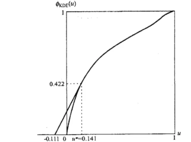
failuretimedistributionin Eq.(24) and

Figure 1: Estimation ofthe optimalagereplacement time basedon the kernel density estimation (Model 1).

$q=0.2$

.

InFig.1,

we

present

an

estimation example of the optimal agereplacement time in Model 1 based

on

thekernel densityestimationfrom 30 observedright-censoreddata,wherethe ideal smoothing parameter

$h$ which maximizes the modified likelihood criterion in Eq.(19) is used. The point providing the steepest

slope among the line segments drawn from $(-\eta_{1},0)=$ -0.111 0) to the scaled TTT transform $\phi \mathrm{K}\mathrm{D}\mathrm{E}(u)$ is

$n’=$ 0.141. Hence,the optimal age replacementtime

can

be estimated

as

$T^{\mathrm{A}}*=$4.025.

Next, let

us

study the asymptotic behavior of two nonparametric estimation algorithms, namely, the

TTT plot using the Kaplan-Meierestimationand the kernel densityestimation. MonteCarlosimulationsare

carriedout with pseudorandom

nrun

bersbased

on

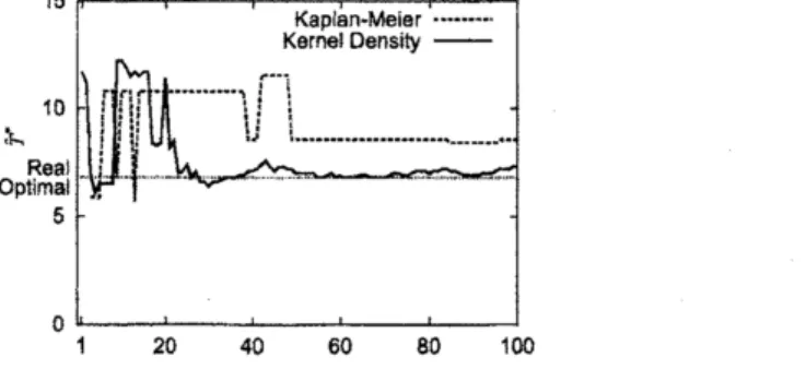
the Weibull failuretime distribution and the exponential

censoring timedistribution,inorder to investigate theconvergencetoward the real optimal solution. Figures

2 to 5 show the asymptotic behavior ofthe optimal age replacement time for Model 1 and 2, From these

figures, it is found that the resultsconverge tothe real optimal solutions when the number of failure time

datais close to30.

Figures6 to 9 show thle

mean

square

error

of estimate of the optimal age replacement time, which

are

obtained

by carryingout the above Monte Carlo simulations

100

times. When the sample size is extremely

small, theestimation accuracy of the kernel density

estimation

is not always high. Once

20

or moresample

data can be obtained, we

can

observe that the estimation accuracy of the optimal age replacement tim

ne

can

be improved by introducing the kernel density estimation. From these results,

we

conclude that the

statisticalalgorithm based

on

the kerneldensityestimation

can

be

recommended

toestimate the optimal age

replacement time,especially for thecensored small sample problem.

7.

Concluding

Remarks

In this paper, we have considered the typical age replacement models

so as

to minimize the relevant

expected costs, and

formulated

thestatistical estimation problems with the censored sample of failure time

data. Based

on

the concept of total time

on

test statistics,

we

haveshownthatthe underlyingoptimization

problems were translated to the graphical

ones on

the data space. Next, we have utilized

a

kernel density

estimator and improve the statistical estimation algorithmsin terms of estimation accuracy. Through the

simulation experiments, it has been shown that the

estimation

accuracy of the kernel density estimation

is higher than the Kaplan-Meier estimation, when the 20

or

more

sample data

can

be obtained. We have

adopted the approach ofmaximizing the modified

likelihood

criterion for the method of determining the

smoothing parameter. In the future effort, it would be interesting to improve the estim ation accuracy by

no.data

Figure2: Asymptotic behavior ofestimateof the optimalage replacement time (Model 1,q$=0.2$).

15 Kaplan-Meier– Kernel Density– 10 $\mathrm{a}_{-}$ $0_{\mathrm{P}^{\mathrm{t}\mathfrak{l}\mathfrak{m}\mathrm{a}1}}^{\mathrm{R}\epsilon \mathrm{a}}5$

$–\sim\dot{}_{*-\cdot m\cdot--\cdot d}’.-\cdot-\cdot-\neg.\mathrm{t}||:\ldots\dot{\lrcorner}:-;\backslash$ $|’\ldots-\cdots.$

.

0

1 20 40 60 80 $\{00$

nodata

Figure3: Asymptotic behavior ofestimateof the optimal age replacement time (Model 1,$q=0.4$).

nodata

Figure4: Asymptotic behavior ofestimate of the optimal age replacement time(Model 2, q$=0.2$).

$\mathrm{n}\mathrm{o}\Delta \mathrm{a}\mathrm{t}\mathrm{a}$

70

Kaplan-Meier $\mathrm{g}$

60 Kemel Density $-arrow-$

so

$\mathrm{b}$ $q)\mathrm{U}\mathrm{J}=4030$ $\prod_{\grave{|},\mathrm{i}_{\Pi}}|[mathring]_{/}$ 20

1’..

$\varpi_{\mathrm{r}\mathrm{J}_{\mathrm{D}}^{*}}^{1}.\tau_{1}$ 10

%\\

$0_{0}$ 10 20 30 40 50 no.data

Figure6: Mean square

error

ofestimate of the optimalagereplacementtime (Model 1, $q=0.2$).

$=\sigma)\mathrm{u}\rfloor$

no.data

Figure7: Mean square

error

ofesti nate of the optimalage replacement time (Model 1, q$=0.4$).

70

Kaplan-Meier 0

60

_’4

KernelDensity $-arrow-$ $50$

$l_{\mathrm{d}}^{4d}|\infty^{\eta-}\mathrm{D}’--|\# 0!_{\Pi^{1}}\beta_{\mathrm{b}}^{\neq \mathrm{l}}$

$\sigma^{\mathrm{J}}\mathrm{u}_{\mathrm{J}}$

$40$ $\cdot \mathrm{o}$ $\mathrm{d}$ $e_{\phi^{\mathfrak{g}}}$

$\alpha^{\mathrm{R}}\mathrm{R}$ $\mathrm{E}$

$2030$

$\mathrm{m}_{3}$

$.-\iota_{\mathrm{h}\backslash _{\mathrm{q}^{-}}^{\mathrm{I}\mathrm{I}}}’\mathrm{r}^{\prime*}\backslash ’+\grave{\#}^{-}$

10

$0_{0}$

{0 20 30 40

so

nodata

Figure8: Mean square

error

ofestimateofthe optimalagereplacement time (Model 2,$q=0.2$).

70 $\mathrm{K}\mathrm{a}\mathrm{p}|\mathrm{a}\mathrm{n}- \mathrm{M}\mathrm{e}\dot{|}\mathrm{e}\mathrm{r}$ $\mathrm{a}$

$6050$ $\Gamma‘.\mathrm{r}_{\backslash }J11$

.

KernelDensity $arrow-$

$\mathrm{t}D\mathrm{u}\mathrm{J}=4030$ $\backslash _{\mathrm{o}^{*\eta}}^{1}\mathrm{i}_{\mathrm{I}}\mathrm{D}\not\in P^{\mathfrak{g}}\mathrm{r}_{\mathrm{p}4_{1}^{\mathrm{f}\mathrm{f}\mathrm{i}^{\mathrm{F}^{\mathrm{o}\mathrm{e}_{\mathrm{E}}}}\mathrm{m}_{\mathrm{Q}}^{d+\mathrm{p}^{\mathrm{g}}}}}l_{)-}\mathrm{b}.\#\}9\mathrm{b}^{\mathrm{m}]}$

20 $\mathrm{r}\cdot[].’\iota_{-}^{-}-I\cdots\neg$

$0 0

0 40 20 30 40 50

no.data

REFERENCES

[1] R.EBarlowand F. Proschan, Mathematical Theory

of

Reliability, John Wiley

&

Sons,New York, (1965).

[2] B. Bergman,Onage replacement and thetotalti

me on

testconcept, Scandinavian Journal

_of

Statistics,

6, PP. 161-168, (1979).

[3] B. Bergman and B. Klefsj6, A graphical method applicable to age-replacement problems, IEEE Trans.

Reliab.,R-31 (5), pp. 478-481, (1982).

[4] B. Bergman and B. Klefsj6, TTT transforms and age replacements withdiscountedcosts, NavalResearch

Logis tics Quarterly, 30, pp. 631-639, (1983).

[5] K. Rinsaka and T.Dohi,Estimatingagereplacement policieswith

a

small sampledata, Proc. 2005

Inter-national Workshop

on

RecentAdvances in Stochastic OperationsResearch, Canmore, Canada, pp.

219-226, 2005

[6] E. Parzen, On the estimation of

a

probability density function and themode, Annals

of

Mathematical

Statistics, 33, pp. 1065-1076, (1962).

[7] M.Rosenblatt, Remarks

on some

nonparametricestimates ofadensity function, Annals

of

Mathematical

Statistics, 27, _PP. 832-837, (1956).

[8] T Cacoullos, Estimation of

a

multivariate density, Annals

of

the Institute

of

Statistical Mathematics,

18, pp 178-189, (1966).

[9] B.W. Silverman, $Derk\mathit{9}\iota ty$ Estimation

for

Statistics and Data Analysis, Chapman and Hall, London,

(1986).

[10|V.A. Epanechnikov, Nonparametric estimation of a multidimensional probability density, Theory

_of

probability andits applications, 14, pp. 153-158, (1969).

[11] $\mathrm{D}.\mathrm{M}$. Reinke, $\mathrm{E}.\mathrm{A}$

.

Pohl and $\mathrm{W}.\mathrm{P}$. Murdock Jr, Survival analysis and maintenance policies for a

series

system, with highly censored data, Proc Annual Reliability and Maintainability Symposium, pp.

182-188, (1998).

[12] $\mathrm{D}.\mathrm{M}$.Reinke,$\mathrm{E}.\mathrm{A}$.Pohl and$\mathrm{W}.\mathrm{P}$

.

MurdockJr, Maintenance-policy cost-analysisfor

a

series system

with

highly-censored data, IEEE Trans. Reliab., R-48(4), pp. 413-420, (1999)

[13] $\mathrm{D}.\mathrm{T}$. McNicholsand$\mathrm{W}.\mathrm{J}$

.

Padgett, Kerneldensity estimation under rando

1ncensorship, Statistics Tech.

Rep.,

no.

74, University ofSouth Carolina, (1981).

[14] $\mathrm{W}.\mathrm{J}$.Padgett, Nonparametric estimation of density and hazard rate

functionswhen samplesarecensored, in Handbook

_of

Statistics, vol. 7 (Edited by$\mathrm{P}$

R. Krishnaiah and$\mathrm{C}.\mathrm{R}$. Rao),pp.313-33, North-Holland,

New York, (1988)

[15] $\mathrm{R}.\mathrm{E}$. Barlow and R. Campo,

Total time

on

testprocesses and applications to failure data, in

Reliabil-ity and Fault Tree Analysis, ed. $\mathrm{R}.\mathrm{E}$. Barlow, J. Pussell and $\mathrm{N}.\mathrm{D}$_, Singpurwalla, pp. 451-48, SIAM,

Philadelphia, (1975).

[16] $\mathrm{B}.\mathrm{L}$

.

Kaplan and P. Meier, Non

parametric estimation from incomplete observations, $J$ A_$mer$, Statist.

Assoc., 53,pp. 457-481, (1958).

[17] $\mathrm{D}.\mathrm{W}$

.

Scott and $\mathrm{L}.\mathrm{E}$

.

Factor, Monte Carlostudy

of three data-based nonparametric probabilitydensity

estimators, J. Amer. Statist Assoc., 76, pp. 9-15, (1981).

[18] L. Leemis, Reliability:

Probabilistic

Models andStatisticalMethods, Prentice-Hall, Englewood Cliffs,$\mathrm{N}.\mathrm{J}$

.