Problems on Low-dimensional Topology, 2018 (Intelligence of Low-dimensional Topology)

Problems on Low‐dimensional Topology, 2018

Edited by T. Ohtsuki1

This is a list of open problems on low‐dimensional topology with expositions of their history, background, significance, or importance. This list was made by editing manuscripts written by contributors of open problems to the problem session of the conference “Intelligence of Low‐dimensional Topology” held at Research Institute for Mathematical Sciences, Kyoto University in May 30— June 1, 2018.

Contents

1 Computational complexity of the colored Jones polynomial at a

root of unity 2

2 The minimal coloring number of\mathbb{Z}_{‐colorable links 3}

3 Triangulations and the 3D _{index of cusped 3‐manifolds 4}

4 Destabilized Heegaard surfaces of 3‐manifolds 5

5 Simplified trisections of 4‐manifolds 6

6 Virtual embeddings between mapping class groups of surfaces 9 7 Totally real immersions and embeddings of n‐manifolds into \mathbb{C}^{n} 11

1Research Institute for Mathematical Sciences, Kyoto University, Sakyo‐ku, Kyoto, 606‐8502, JAPAN

Email: [email protected]‐u.ac.jp

1

Computational complexity of the colored Jones polyno‐

mial at a root of unity

(Oliver Dasbach)

The volume conjecture of Kashaev and Murakami & Murakami and its gen‐ eralizations connect the growth of evaluations of the colored Jones polynomial

J_{N}(L;e^{2\pi\sqrt{-1}/N})

of a link L _{to geometric information of its link complement. For}

J_{2}(L;q), i.e. the classical Jones polynomial, it is known by a result of Jaeger, Ver‐

tigan and Welsh [32, 61] that evaluations at all but eight points (2nd, 3rd, 4th, 6th

roots of unity) are \#P‐hard. At those eight points polynomial time algorithms are known (see the second remark below), in particular for J_{2}(L;-1) .

Question 1.1 (O. Dasbach). What can one say about the computational complexity

of

J_{N}(L;e^{2\pi\sqrt{-1}/N})

for N=5 _and N\geq 7^{i)}

Remark. It is known (see e.g. [50]) that the colored Jones polynomial J_{N}(K;q) of a knot K _{can be presented by a linear sum of the Jones polynomial}

_{J_{2}(K^{(n)};q)}

_of

K^{(n)} _{(for n=1,2,} \cdots

, N-1_{), where} K^{(n)} _{denotes the union of} n parallel copies of K_{. Similarly, J_{N}(L;q) of a link} L _{can be presented by a linear sum of the Jones}

polynomial of links obtained from L _{by replacing each component with parallel}

copies of it. Further, it is known (see the remark below) that the Jones polynomial can be calculated in polynomial time at 2nd, 3rd, 4th, 6th roots of unity. Hence,

when N=2,3,4,6,

J_{N}(L;e^{2\pi\sqrt{-1}/N})

can be calculated in polynomial time.

Remark. At a 2nd, 3rd, 4th, 6th root of unity, the Jones polynomial of a link L _can

be calculated in polynomial time of the number of crossings of a diagram of L _in

the following ways. It can be shown by a skein relation that

J_{2}(L;1)=(-2)^{\# L-1}

and

J_{2}(L;e^{2\pi\sqrt{-1}/3})=1

, where \# L denotes the number of components of L_{. It is}

known that |J_{2}(L;-1)| is equal to the order of

_{H_{1}(M_{2,L})}

if its order is finite, and

0 _{otherwise, where M_{2,L} denotes the double branched cover of} S^{3} _{branched along}

L_{. It is known [49] that}

J_{2}(L;\sqrt{-1})=(-\sqrt{2})^{\# L-1}(-1)^{Arf(L)}

_{if Arf(L) exists, and} 0 _{otherwise. It is known [43] that}

J_{2}(L;e^{\pi\sqrt{-1}/3})=\pm\sqrt{-1}^{\# L-1}\sqrt{-3}^{\dim H_{1}(M_{2,L},\mathbb{Z}/3\mathbb{Z})}

By using such topological interpretations, the Jones polynomial can be calculated in polynomial time at 2nd, 3rd, 4th, 6th roots of unity.

When q is not such a root of unity, it is known [32, 61] that computing J_{2}(L;q)

of an alternating link L _{is \#P‐hard.}

The following remark is due to Tetsuya Ito.

Remark (T. Ito). It is known [30] that the invariants of Question 1.1 can be presented by the colored Alexander invariants, which are defined by homological representa‐ tions of the braid groups generalizing the Burau representation. By using these invariants, the invariants of Question 1.1 can be calculated in polynomial time, and Question 1.1 is solved affirmatively.

2

The minimal coloring number of

\mathbb{Z}

_{‐colorable links}

(Kazuhiro Ichihara2 and Eri Matsudo3)

The Fox n‐coloring would be one of the most well‐known invariants of knots and

links (

n\geq 2

_{an integer). However, some of links are known to admit non‐trivial Fox}

n

‐colorings for every

n\geq 2

, that is, the links with

0

determinants (see the remark

at the end of this section). For such a link, we can define a \mathbb{Z}_{‐coloring as follows,}

which is a natural generalization of the Fox n‐coloring.

Let L _{be a link and} D _{a regular diagram of} L_{. A map} \gamma from the set of the arcs

of D_to \mathbb{Z}_{is called a} \mathbb{Z}_{‐coloring on} D _{if it satisfies the condition 2\gamma(a)=\gamma(b)+\gamma(c)}

at each crossing of D _{with the over arc} a and the under arcs b and c. A\mathbb{Z}‐coloring

which assigns the same integer to all the arcs of the diagram is called the trivial

\mathbb{Z}_{‐coloring. A link is called} \mathbb{Z}_{‐colorable if it has a diagram admitting a non‐trivial} \mathbb{Z}_{‐coloring. (As usual, we call the integers appearing in the image of a} \mathbb{Z}_‐coloring

the colors.)

For a \mathbb{Z}_{‐colorable link} L_{, the minimal coloring number of a diagram} D _of L _is

defined as the minimal number of the colors for all non‐trivial \mathbb{Z}_{‐colorings on D,}

and the minimal coloring number of L _{is defined as the minimum of the minimal}

coloring numbers of diagrams representing the link L.

The minimal numbers of colors for knots and links admitting Fox’s colorings behave interestingly, and have been studied in detail recently. On the other hand,

the following was shown by the second author in [47] and by Meiqiao Zhang, Xian’an

Jin and Qingying Deng in [62] independently, based on the result given in [27].

Theorem ([62], [47]) The minimal coloring number of any non‐splittable \mathbb{Z}_‐colorable

link is equal to 4.

We here remark that the proofs in both [47] and [62] are quite algorithmic, and

so, the resultant diagrams in their proofs admitting a \mathbb{Z}_{‐coloring with four colors}

are often very complicated.

In view of this, in [28], we have considered and studied the minimal coloring

numbers of minimal diagrams of \mathbb{Z}_{‐colorable links, that is, the diagrams representing}

the link with least number of crossings.

Based on the results obtained in [28], the following problems can be considered.

Problem 2.1 (K. Ichihara, E. Matsudo). Determine the minimal coloring number

of minimal diagrams of \mathbb{Z}_{‐colorable torus links.}

Remark. It is known that which torus links admit non‐trivial \mathbb{Z}_{‐colorings. See [1] for}

example to compute the determinants of torus links. In [28, Theorem 1.3], we showed that, for even integer n>2 _{and non‐zero integer p, the torus link T(pn, n) has a}

minimal diagram admitting a \mathbb{Z}_{‐coloring with only four colors. We have studied}

several other cases, but not obtained the complete classification yet.

2Department of Mathematics, College of Humanities and Sciences, Nihon University, 3‐25‐40 Sakurajosui,

Setagaya‐ku, Tokyo 156‐8550, Japan

Email address: ichihara@math. chs.nihon‐u. ac.jp

Email a

ddress:[email protected]\circ n-uac.jp8550,Japan3

Graduate School o

fI

Problem 2.2 (K. Ichihara, E. Matsudo). Determine the minimal coloring number of minimal diagrams of \mathbb{Z}_{‐colorable pretzel links.}

Remark. It is also known that which pretzel links admit non‐trivial \mathbb{Z}_{‐colorings. See}

[14] to compute their determinants. In [28], we also obtained some results for such links, but not obtained the complete classification yet.

Remark. A topological interpretation of a \mathbb{Z}_{‐coloring is a homomorphism}

L)arrow Aut(\mathbb{Z}), where we denote by Aut(\mathbb{Z}) the subgroup of Map (\mathbb{Z}, \mathbb{Z}) generated by f_{a} (for a\in \mathbb{Z}_{) given by f_{a}(x)=2a-x. This homomorphism naturally induces}

a homomorphism

H_{1}(M_{2,L};\mathbb{Z})arrow 2\mathbb{Z}

, where M_{2,L} denotes the double cover of S^{3}

branched along L_{. We note that} \mathbb{Z} _{naturally acts on the set of} \mathbb{Z}_{‐colorings by}

adding a constant to all colors of a coloring. We have a natural bijection

{

\mathbb{Z}

_{‐colorings of a diagram of}

L

_{} /\mathbb{Z}arrow Hom(H_{1}(M_{2,L};\mathbb{Z}), 2\mathbb{Z}) .}

The determinant of L _{is the determinant of a presentation matrix of}

_{H_{1}(M_{2,L})}

_(see e.g.

[42])

. Hence, when the determinant of L is 0, the rank of

H_{1}(M_{2,L})

is positive,

and we have non‐trivial \mathbb{Z}_{‐colorings of} L.

3

Triangulations and the

3D

_{index of cusped 3‐manifolds}

(Neil Hoffman)

Let (M, T) be an cusped, orientable 3‐manifold and T _{be an ideal triangulation}

of M_{. We say} T _{is 1‐efficient if the only embedded normal surfaces in} T _with

non‐negative Euler characteristic are the boundary linking tori (made up solely of triangular disks). In our context, we say a triangulation is 0_{‐efficient if there are}

no embedded normal S^{2} _or RP^{2}_{. The concept of} 0_{‐efficient and 1‐efficient trian‐}

gulations was introduced by Jaco and Rubinstein [31] and they were able to show

that any triangulation of an irreducible manifold can be algorithmically simplified

to 0‐efficient one.

The

3D

_{‐index is an invariant introduced by Dimofte, Gaiotto and Gukov [15],}

which associated to a 1‐effcient ideal triangulation of a 3‐manifold with torus bound‐ ary components. Furthermore, if two 1‐efficient triangulations are associated by a

2/3, 3/2, 0/2 or 2/0 Pachner move, then the

3D

_{‐indices of both triangulations are}

identical by work of Garoufalidis, Hodgson, Rubinstein and Segerman [20]. This motivates the following question which appears in [19] and in discussed in Section 12 of that paper:

Question 3.1 (S. Garoufalidis, C.D. Hodgson, N.R. Hoffman, J.H. Rubinstein [19]). Given a cusped, atoroidal 3‐manifold M. Are all 1‐eficient triangulations connected by 2/3, 3/2, 0/2 or 2/0 Pachner moves ‘?

It is worth mentioning that a more basic question is also appears to be open. Question 3.2 (folklore). Given a cusped, irreducible 3‐manifold M. Are all 1‐ efficient triangulations connected by 2/3, 3/2, 0/2 or 2/0 Pachner moves?

Henry Segerman showed that triangulations without degree 1 edges are connected in the Pachner graph [56]. The absence of degree 1 edges is a necessary condition for a triangulation to be 0_{‐efficient.}

There is also a version of the 3D _{index which associates to each peripheral curve}

a formal Laurent series. Suggesting that closed manifolds may be assigned a 3D

index in this way.

Question 3.3 (N. Hoffman). Is this assignment a topological invariant9 That is given two different Dehn surgery presentations of the same manifold, will the 3D

index for each presentation be the sam e^{}

A lighter version of this question was asked by Dongmin Gang [18].

Conjecture 3.4 (D. Gang [18]). If the 3D _{index evaluated on a slope is an infinite}

series starting with 1+\cdots, if the Dehn filling corresponds to a hyperbolic 3‐manifold

and the

3D

_{index is}

_0,1

_or

\infty

(does not converge), if

M

is non‐hyperbolic. In

particular, if the Dehn filling is a lens space, then the 3D _{index is} 0

We remark that Gang’s conjecture is supported by a number of a computations. Finally, let infinite collection of Dehn fillings

_{\{M_{\gamma_{\dot{i}}}\}}

of a cusped manifold M _such

that the geometric limit of the

\{M_{\gamma_{i}}\}

is M.

Question 3.5 (N. Hoffman). Is there a normalization for the 3D _{index such that}

a sequence of 3D _{indices computed on the}

_{\{M_{\gamma_{\dot{i}}}\}}

_{converges (term‐wise) to the} 3D

index of M^{t}_?

4

Destabilized Heegaard surfaces of 3‐manifolds

(Yeonhee Jang, Tsuyoshi Kobayashi, Makoto Ozawa and Kazuto Takao) We briefly recall some of the standard terminology and facts. A Heegaard surface

of a 3‐manifold is an embedded closed surface which divides the manifold into two

handlebodies. It is an important fact that every closed orientable 3‐manifold has a Heegaard surface. For a given Heegaard surface, we can construct a new Heegaard surface of the same 3‐manifold by adding a canceling pair of handles. A Heegaard surface is said to be destabilized if it cannot be produced by this construction.

The following is a general problem.

Problem 4.1. Classify the Heegaard surfaces of each closed orientable 3‐manifold. In particular, classifying the destabilized ones is an essential part.

We briefly review some of the abundant known results for the above problem. Waldhausen [60] showed the uniqueness of destabilized Heegaard surfaces of the 3‐

sphere, and Bonahon and Otal [10, 11] showed that of lens spaces. Hence, if there is

a Heegaard surface of genus 0 _{or 1, then the destabilized ones of the 3‐manifold are}

unique. On the other hand, Casson‐Gordon (see [48, 54]) and Moriah‐Schleimer‐

Sedgwick [48] gave families of 3‐manifolds each of which has infinitely many destabi‐

lized Heegaard surfaces of pairwise distinct genera. The minimal genus of Casson‐ Gordon’s Heegaard surfaces is 4, and that of Moriah−Schleimer−Sedgwick’s is 3,

though we do not know whether they attain the minimums of the manifolds. We

also refer the reader to [53, 58] for a theorem on the stable equivalence, to [33, 40]

for theorems on the finiteness at any given genus, to [13, 36, 41] for classification algorithms, and to [25, 35, 38, 45, 55] for relevant examples.

The following is one of various open problems suggested by the above results. Problem 4.2. Prove or disprove the existence of a 3‐manifold which has a Heegaard surface of genus 2, and infinitely many destabilized ones of pairwise distinct genera.

5

Simplified trisections of 4‐manifolds

(Osamu Saeki4)

A trisection of a 4‐manifold was introduced by Gay‐Kirby [21], and it is expected to be a generalization of a Heegaard splitting of a 3‐manifold. Roughly speaking, a trisection of a 4‐manifold M _{is a decomposition M=M_{1}\cup M_{2}\cup M_{3} such that}

for a fixed non‐negative integer \ell, M_{i} is diffeomorphic to

\Vert^{\ell}(S^{1}\cross B^{3})(4

‐dimensional handlebody) for i=1,2,3, and M_{1}\cap M_{2}\cap M_{3} is a closed orientable surface of genus

g, and

X_{k}=(M_{k}\cap M_{i})\cup(M_{k}\cap M_{j})

is a 3‐manifold having a Heegaard splitting of

genus gas the union of M_{k}\cap M_{i} and M_{k}\cap M_{j}for \{k, i, j\}=\{1,2,3\}. As a Heegaard

splitting of a 3‐manifold X _{can be studied by using a Morse function Xarrow \mathbb{R},} a

trisection of a 4‐manifold M _{can be studied by using a Morse 2‐fUnction} Marrow \mathbb{R}^{2}.

Let M _{be a smooth closed connected oriented 4‐manifold. A smooth map f :}

Marrow \mathbb{R}^{2} _{is a trisected Morse 2‐function (or a trisection map) if it has only fold and}

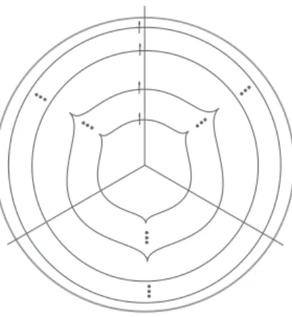
cusp singularities and it satisfies the following conditions (see [21, 8, 9] and Fig. 1):

(1) its image is diffeomorphic to a 2‐disk, denoted by D^{2},

(2) it has a single definite fold circle mapped diffeomorphically onto the boundary

\partial D^{2} of _D^{2},

(3)

D^{2}\backslash \{p\}

can be nonsingularly foliated by rays from a regular value p to \partial D^{2},

each intersecting the indefinite fold image always in the direction of index‐2 handle attachments,

(4) three of these rays split D^{2} _{into three sectors, where there is at most one cusp}

on each singular arc image in a sector,

(5) the total number of cusps in the sectors are equal,

(6) the singular arcs with cusps are situated inside.

The number gof indefinite fold arcs (possibly with a cusp) in each sector is called

the genus of the trisection. Note that

f^{-1}(p)

is a closed orientable surface of genus

g for the regular value p\in D^{2}.

It is known that for every trisection decomposition of M_{, there is a trisected}

Morse 2‐function f : Marrow \mathbb{R}^{2} _{which gives the given trisection decomposition.}

Email a

_{ddress:[email protected]\dot{{\imath}}}

tute o

fMathemat\dot{{\imath}}csforI

Figure 1: The figure on the left depicts the image of a trisected Morse 2‐function. In each box there is an arbitrary Cerf graphic as in the right [21, §3]. The three half lines divide the image into three parts and their inverse images correspond to 4‐dimensional handlebodies giving a trisection decomposition.

As far as the author knows, the following problem is still open.

Problem 5.1 (R.I. Baykur, O. Saeki [8]). Non‐isotopic trisected Morse 2‐functions may yield equivalent trisection decompositions. Describe the necessary and sufficient conditions for two trisected Morse 2‐functions to give equivalent trisection decompo‐

sitions.

A trisection is said to be simplified if there exists an associated trisection map

such that the restriction to its singular locus is an embedding [8, 9] (see Fig. 2).

This is in great contrast with a general trisection map (see Fig. 1), which has Cerf boxes in between the three sectors of the image 2‐disk, where folds can cross each other arbitrarily (and therefore, the images of some indefinite fold circles might wind around p multiple times).

Note that Hayano [26] has studied the condition for a given trisection decom‐ position to be equivalent to a simple one. He has also classified genus‐2 simplified

trisections.

The following manifolds are known to admit genus‐3 simplified trisections [9]:

S^{4}, connected sums of \mathbb{C}\mathbb{P}^{2}, \overline{\mathbb{C}\mathbb{P}}^{2} _and S^{1}\cross S^{3} _{with three summands, connected sum}

of either one of these manifolds with S^{2}\cross S^{2}_{, Pao’s manifolds L_{n},}

_{L_{n}'[51]}

_{. One}

can similarly get genus‐4 examples on connected sums of lower genera trisections on these standard 4‐manifolds. In addition, we have the irreducible examples on L(p, q)‐bundles and

(S^{1}\cross S^{2})

‐bundles over S^{1}_{, which include} S^{2}_{‐bundles over the}

2‐torus T^{2} and the Klein bottle Kb.

The following two problems have been posed in [9].

Problem 5.2 (R.I. Baykur, O. Saeki [9]). Classify 4‐manifolds that admit simplified genus‐3 trisections. Is there any 4‐manifold, other than the ones mentioned above, which admits genus‐3 simplified trisections l

Figure 2: Singular value of a simplified trisected Morse 2‐function

Question 5.3 (R.I. Baykur, O. Saeki [9]). Is there any 4‐manifold which admits a

trisection, but not a simplified one of the same genus /? Defining the minimal tri‐ section genus ( re\mathcal{S}p. minimal simplified trisection genus) of a 4‐manifold M as the

smallest genus of a trisection (resp. simplified trisection) on M_{, one can equiva‐}

lently ask if there is a 4‐manifold whose trisection genus is strictly smaller than its simplified trisection genus.

The two genera are equal for all of the 4‐manifolds with (simplified) trisections of genus g\leq 4 mentioned above. The answer to the analogous question for broken Lefschetz fibrations versus simplified broken Lefschetz fibrations is positive [7].

Heegaard splittings of a closed oriented 3‐manifold X _{are closely related with a}

Morse function g:Xarrow \mathbb{R}. Based on this, Johnson [34] and Takao [59] used generic maps into \mathbb{R}\cross \mathbb{R}=\mathbb{R}^{2} _{for comparing two Heegaard splittings of a given 3‐manifold.}

Question 5.4 (O. Saeki). Can we use a similar idea for comparing two trisections of a given 4‐manifold to get some information on the relationship between the two

trisections /?

It is well known that any two Heegaard splittings of a given 3‐manifold are

related by a sequence of stabilizations. As an analog, it is shown [21] that any two

trisections of a given 4‐manifold are related by a sequence of “stabilizations” In

[21], this is proved by using handle decompositions of a 4‐manifold and stabilizations

of Heegaard splittings of 3‐manifolds.

Problem 5.5 (D. Gay, R. Kirby [21]). Find a singularity theoretical proof of the uniqueness of trisections (up to stabilization) on a given 4‐manifold.

6

Virtual embeddings between mapping class groups of sur‐

faces

(Takuya Katayama)

Let

_{\Sigma_{g,p}^{b}}

be a compact orientable surface of genus g with p marked points and

b_{boundary components. The mapping class group (or Teichmüller modular group)}

Mod

_{(\Sigma_{g,p}^{b})}

of

_{\Sigma_{g,p}^{b}}

is the group of orientation‐preserving homeomorphisms of

_{\Sigma_{g,p}^{b}}

fixing the set of marked points setwise and fixing the boundary pointwise, up to isotopy relative to the marked points and the boundary. In particular, Mod

_{(\Sigma_{0,n}^{1})}

is naturally identified with the nth braid group B_{n}.

Homomorphisms between mapping class groups have been studied in many re‐ searches. A typical construction of such a homomorphism is induced by an embed‐ ding of a surface, i. e., a combination of forgetting marked points, deleting bound‐ ary components, and subsurface embeddings; see [4]. Another typical construction of such a homomorphism is induced by a covering of a surface. For example, a

natural double branched covering

_{\Sigma_{2,0}^{0}arrow\Sigma_{0,6}^{0}}

induces a surjective homomorphism

Mod

(\Sigma_{2,0}^{0})arrow Mod(\Sigma_{0,6}^{0})

, whose kernel is a cyclic group of order 2; see [46]. Further,

natural double coverings

_{\Sigma_{g,0}^{1}arrow\Sigma_{0,2g+1}^{1}}

and

_{\Sigma_{g,0}^{2}arrow\Sigma_{0,2g+2}^{1}}

induce injective homo‐

morphisms

B_{2g+1}arrow Mod(\Sigma_{g,0}^{1})

and

B_{2g+2}arrow Mod(\Sigma_{g,0}^{2})

; see [16, Section 9.4]. The

topic of homomorphisms between mapping class groups is related to the rigidity of

structures on surfaces; see [5] for a survey on this topic.

Moreover, injective homomorphisms between mapping class groups have also been studied in some researches. By modifying the above mentioned homomorphisms of B_{2g+1} and B_{2g+2}, we can obtain injective homomorphisms

_{B_{2g+1}arrow Mod(\Sigma_{g+1,0}^{0})}

and

_{B_{2g+2}arrow Mod(\Sigma_{g+1,0}^{0})}

; see [24, 37]. Further, it is known [3] that, for any

g\geq 2, there exist g'>g and an injective homomorphism Mod

_{(\Sigma_{g,0}^{0})arrow Mod(\Sigma_{g,0}^{0})}

. On the other hand, it is known [24] that, when g\geq 3and g>g', there are no nontrivial homomorphisms Mod

_{(\Sigma_{g,0}^{0})arrow Mod(\Sigma_{g,0}^{0})}

.

We say that a group H_{is embedded in another group} G_{if there exists an injective}

homomorphism from H_to G_{. Further, as in [6], we say that} H_{is virtually embedded}

in G_{if a finite index subgroup of} H_{is embedded in} G_{. We note that the composition}

of virtual embeddings is a virtual embedding.

As an example of a virtual embedding, we can show that Mod

_{(\Sigma_{2,0}^{0})}

is virtually embedded in Mod

_{(\Sigma_{0,6}^{0})}

, as follows. As mentioned above, a double covering

_{\Sigma_{2,0}^{0}arrow}

\Sigma_{0,6}^{0}

induces a homomorphism Mod

_{(\Sigma_{2,0}^{0})arrow Mod(\Sigma_{0,6}^{0})}

whose kernel is a cyclic group of order 2 (generated by the hyperelliptic involution \iota). Since Mod

(\Sigma_{2,0}^{0})

is residually finite (see [16, Section 6.4]), we can find a finite index subgroup H _of

Mod

_{(\Sigma_{2,0}^{0})}

such that the restriction map

_{Harrow Mod(\Sigma_{0,6}^{0})}

is injective, by showing that its kernel \{1, \iota\}\cap H is trivial. Hence, Mod

_{(\Sigma_{2,0}^{0})}

is virtually embedded in Mod

_{(\Sigma_{0,6}^{0})}

. This construction is a topological interpretation of a virtual embedding. See also [57, Theorem 2] for a preceding result on virtual embeddings.

Problem 6.1 (T. Katayama). Given g\geq 2, determine whether Mod

_{(\Sigma_{g,0}^{0})}

is virtu‐ ally embedded in Mod

(\Sigma_{g,p}^{b'},)

.

Remark 1. If g was 1, we can show that it is relatively easy to make a virtual

embedding of Mod

_{(\Sigma_{1,0}^{0})}

to a mapping class group, as follows. It is known, see e.g.

[44, Proposition 4.4.2], that Mod

(\Sigma_{1,0}^{0})

is SL(2;\mathbb{Z}) and it has the rank 2 free group as a finite index subgroup. Further, we can embed the rank 2 free group into almost all mapping class groups, by considering Dehn twists along two essential simple closed curves with at least two crossings; see [29]. Hence, if g was 1, Problem 6.1 would be

relatively easy.

Remark 2. When g=2, we can show that Mod

_{(\Sigma_{2,0}^{0})}

is virtually embedded in

Mod

_{(\Sigma_{g,0}^{0})}

for any g'\geq 3 , as follows. As mentioned above, Mod

_{(\Sigma_{2,0}^{0})}

is virtually

embedded in Mod

_{(\Sigma_{0,6}^{0})}

. Further, by Remarks 2A _and 2B _{below, Mod}

_{(\Sigma_{0,6}^{0})}

_is

virtually embedded in Mod

_{(\Sigma_{g,0}^{0})}

for any g'\geq 3 . Hence, Mod

_{(\Sigma_{2,0}^{0})}

is virtually embedded in Mod

_{(\Sigma_{g,0}^{0})}

for any g'\geq 3.

Therefore, when g=2, g'\geq 3 and p'+b'=0 , Problem 6.1 is solved affirmatively. It is not known whether Mod

_{(\Sigma_{g,0}^{0})}

is virtually embedded in Mod

_{(\Sigma_{g,p}^{b},)}

, when g\geq 3

or p'+b'\geq 1.

Remark 2A_{. We can show that Mod}

_{(\Sigma_{0,6}^{0})}

_{is virtually embedded in B_{5}, as fol‐}

lows. It is known [12, Theorem 10] that the pure braid group P_{5} is isomorphic to PMod

_{(\Sigma_{0,6}^{0})\cross \mathbb{Z}}

, where PMod

_{(\Sigma_{0,6}^{0})}

is the finite index subgroup of Mod

_{(\Sigma_{0,6}^{0})}

fixing the marked points. Since there is an embedding PMod

_{(\Sigma_{0,6}^{0})arrow P_{5}arrow B_{5},}

Mod

_{(\Sigma_{0,6}^{0})}

is virtually embedded in B_{5}.

Remark 2B_{. We can show that B_{5} is embedded in Mod}

_{(\Sigma_{g,0}^{0})}

_{for any g\geq 3, as}

follows. As mentioned before, there is an embedding

_{B_{2g+1}arrow Mod(\Sigma_{g+1,0}^{0})}

. Hence,

when g\geq 3, there is an embedding

_{B_{5}arrow B_{2g-1}arrow Mod(\Sigma_{g,0}^{0})}

. Therefore, B_{5} is

embedded in Mod

_{(\Sigma_{g,0}^{0})}

for any g\geq 3.

Remark 3. It is known [37, Corollary 1.7] that, when

g, g'\geq 2,

Mod(\Sigma_{g,p}^{0})

is virtually

embedded in Mod

_{(\Sigma_{g,p}^{0},)}

, only if 3g+p\leq 3g'+p' and 2g+p\leq 2g'+p'.

It follows from [4, Corollary 1.2] that, if 6\leq g<g'\leq 2g-2,

_{Mod(\Sigma_{g,0}^{0})}

is not

embedded in Mod

_{(\Sigma_{g,0}^{0})}

.

It is known [4, Proposition 7.1] that, if

g\geq 3

and

g>g'

, any homomorphism

Mod

_{(\Sigma_{g,p}^{b})arrow Mod(\Sigma_{g,p}^{b},)}

is trivial.

Conjecture 6.2 (T. Katayama). Suppose that g\geq 2. If Mod

_{(\Sigma_{g,p}^{b})}

is virtually embedded in B_{n} for some n, then (g,p, b)=(2,0,0).

When (g,p, b)=(2,0,0), we note that Mod

_{(\Sigma_{2,0}^{0})}

is virtually embedded in B_{5} by

Remarks 2 and 2A of Problem 6.1.

In case there is a counter‐example to Conjecture 6.2, the target braid group does not admit faithful C^{\infty} _{action on} \mathbb{R}_{even virtually, and is not “virtually special” (i.e.,}

no finite index subgroup is embedded in a right‐angled Artin group, see [6, Question 2] ) .

Problem 6.3 (T. Katayama). Find a pair

(H, \phi)

of a finite index subgroup

H

_of

Mod

_{(\Sigma_{g,p}^{b})}

and a homomorphism

_{\phi:Harrow Mod(\Sigma_{g,p}^{b},)}

with t

Remark. Some “surface manipulations” induce homomorphisms with “small kernels” (see [3], [4], [16, Chapter 3], [46] and [52]). Are there any other homomorphisms

with “small kernels”?

7

Totally real immersions and embeddings of

n

‐manifolds

into \mathbb{C}^{n}

(Naohiko Kasuya5)

Let M^{n} be a closed orientable n‐manifold and f:M^{n}arrow \mathbb{C}^{n} be an immersion.

A point p\in M^{n} is said to be a complex tangent if

df_{p}(T_{p}M^{n})

contains a complex line. An immersion is said to be totally real if it has no complex tangent. It follows from Thom’s transversality theorem that the set of complex tangents of a generic immersion f:M^{n}arrow \mathbb{C}^{n} is empty or forms a closed (n-2)‐dimensional submanifold. For totally real immersions and embeddings, the following theorems are known. These are called the h_{‐principle for totally real immersions and embeddings.}

Theorem (Gromov [22], Lees [39]). An n‐manifold M^{n} admits a totally real immer‐

sion into \mathbb{C}^{n} _{if and only if the complexified tangent bundle} \mathbb{C}TM^{n} _{is trivial.}

Theorem (Gromov [23], Forstnerič [17]). Let M^{n} _{be a closed orientable} n‐manifold

with n\geq 3. Then, M^{n} _{admits a totally real embedding into} \mathbb{C}^{n} _{if and only if it}

admits a totally real immersion into \mathbb{C}^{n} _{which is regularly homotopic to an embed‐}

ding.

In the following, we consider the case where n=3_{. It follows from the h‐}

principle that any closed orientable 3‐manifold admits a totally real embedding into

\mathbb{C}^{3}_{. However, there are few explicit examples of totally real embeddings. The}

following example is due to Ahern and Rudin.

Example (Ahern‐Rudin [2]). Let

P(z, w)=\overline{z}\overline{w}(|w|^{2}+i|z|^{2})

. We consider the 3‐ sphere as the unit sphere

_{S^{3}=\{(z, w)||z|^{2}+|w|^{2}=1\}\subset \mathbb{C}^{2}}

. Then, the embedding

f:S^{3}arrow \mathbb{C}^{3}

defined by

f(z, w)=(z, w, P(z, w))

is a totally real embedding.

Inspired by their example, Forstnerič constructed some other examples of totally real embeddings of quotients of the 3‐sphere, including \mathbb{R}P^{3}_{. But we want more}

examples.

Problem 7.1 (N. Kasuya). Construct interesting examples of totally real embed‐

dings of 3‐manifolds into

\mathbb{C}^{3}

_{(without using the}

h

_{‐principle). For example, can a}

Haefliger knot be explicitly realized as a totally real submanifold of \mathbb{C}^{3_{i)}}.

References

[1] Ahara, K., Watanabe, S., Goeritz invariant of torus links, preprint, arXiv:1312.7531

[2] Ahern, P., Rudin, W., Totally real embeddings of S^{3} _in \mathbb{C}^{3}_{, Proc. Amer. Math. Soc. 94 (1985)}

460‐462.

[3] Aramayona, J., Leiniger, C., Souto, J., Injections of mapping class groups, Geom. Topol. 13 (2009) 2523‐2541.

[4] Aramayona, J., Souto, J., Homomorphisms between mapping class groups, Geom. Topol. 16 (2012) 2285‐2341.

[5] —, Rigidity phenomena in the mapping class group, Handbook of Teichmüller theory.

Vol. VI, 131‐165, IRMA Lect. Math. Theor. Phys. 27, Eur. Math. Soc., Zürich, 2016.

[6] Baik, H., Kim, S., Koberda, T., Unsoomthable group action on compact one‐manifolds,

arXiv: 1601. 05490v3.

[7] Baykur, R. I., Broken Lefschetz fibrations and smooth structures on 4‐manifolds, Geom. Topol. Monogr. 18 (2012) 312‐317.

[8] Baykur, R. I., Saeki, O., Simplifying indefinite fibrations on 4‐manifolds, arxiv:1705.11169.

[9] —, Simplified broken Lefschetz fibrations and trisections of 4‐manifolds,

arXiv:1710.06529, to appear in Proc. Natl. Acad. Sci. USA.

[10] Bonahon, F., Difféotopies des espaces lenticulaires, Topology 22 (1983) 305‐314.

[11] Bonahon, F., Otal, J.‐P., Scindements de Heegaard des espaces lenticulaires, Ann. Sci. École

Norm. Sup. (4) 16 (1983) 451‐466.

[12] Clay, M., Leininger, C. J., Margalit, D., Abstract commensurators of right‐angled Artin groups and mapping class groups, Math. Res. Lett. 21 (2014) 461‐467.

[13] Colding, T. H., Gabai, D., Ketover, D., On the classification of Heegaard splittings,

arXiv: 1509.05945.

[14] Dasbach, O. T., Futer, D., Kalfagianni, E., Lin, X.‐S., Stoltzfus, N. W., Alternating sum

formulae for the determinant and other link invariants, J. Knot Theory Ramifications 19

(2010) 765‐782.

[15] Dimofte, T., Gaiotto, D., Gukov, S., 3‐manifolds and 3d indices, Adv. Theor. Math. Phys. 17 (2013) 975‐1076.

[16] Farb, B., Margalit, D., A primer on mapping class groups, Princeton Mathematical Series 49, Princeton University Press, Princeton, NJ, 2012.

[17] Forstnerič, F., On totally real embeddings into \mathbb{C}^{n}_{, Exposition. Math. 4 (1986) 243‐255.}

[1S] Gang, D., Quantum approach to Dehn surgery problem, arXiv:1803.11143.

[19] Garoufalidis, S., Hodgson, C. D., Hoffman, N. R., Rubinstein, J. H., The 3D_{‐index and normal}

surfaces, Illinois J. Math. 60 (2016) 289‐352.

[20] Garoufalidis, S., Hodgson, C. D., Rubinstein, J. H., Segerman, H., 1‐effcient triangulations and the index of a cusped hyperbolic 3‐manifold, Geom. Topol. 19 (2015) 2619‐2689. [21] Gay, D., Kirby, R., Trisecting 4‐manifolds, Geom. Topol. 20 (2016) 3097‐3132.

[22] Gromov, M. L. A topological technique for the construction of solutions of differential equations and inequalities, Proceedings ICM (Nice 1970), vol. 2 (1971) 221‐225.

[23] —, Partial differential relations, Ergebnisse der Mathematik und ihrer Grenzgebiete (3) [Results in Mathematics and Related Areas (3)], 9. Springer‐Verlag, Berlin, 1986.

[24] Harvey, W., Korkmaz, M., Homomorphisms from mapping class groups, Bull. London Math. Soc. 37 (2005) 275‐284.

[25] Hass, J., Thompson, A., Thurston, W., Stabilization of Heegaard splittings, Geom. Topol. 13 (2009) 2029‐2050.

[26] Hayano, K., On diagrams of simplified trisections and mapping class groups, arXiv:1711.02790.

[27] Ichihara, K., Matsudo, E., Minimal coloring number for \mathbb{Z}_{‐colorable links J. Knot Theory}

Ramifications 26 (2017) 1750018, 23 pp.

[28] —, Minimal coloring number on minimal diagrams for \mathbb{Z}_{‐colorable links, Proceedings of}

the Institute of Natural Sciences, Nihon University 53 (2018) 231‐237.

[29] Ishida, A., The structure of subgroup of mapping class groups generated by two Dehn twists, Proc. Japan Acad. Ser. A Math. Sci. 72 (1996) 240‐241.

[30] Ito, T., A homological representation formula of colored Alexander invariants, Adv. Math. 289 (2016) 142‐160.

[31] Jaco, W., Rubinstein, J. H., 0_{‐efficient triangulations of 3‐manifolds, J. Differential Geom. 65}

(2003) 61‐168.

[32] Jaeger, F., Vertigan, D. L., Welsh, D. J. A., On the computational complexity of the Jones and Tutte polynomials, Math. Proc. Cambridge Philos. Soc. 108 (1990) 35‐53.

[33] Johannson, K., Heegaard surfaces in Haken 3‐manifolds, Bull. Amer. Math. Soc. (N.S.) 23 (1990) 91‐98.

[34] Johnson, J., Stable functions and common stabilizations of Heegaard splittings, Trans. Amer. Math. Soc. 361 (2009) 3747‐3765.

[35] —, Bounding the stable genera of Heegaard splittings from below, J. Topol. 3 (2010)

668‐690.

[36] —, Calculating isotopy classes of Heegaard splittings, arXiv:1004.4669.

[37] Katayama, T., Kuno, E., The RAAGs on the complement graphs of path graphs in mapping class groups, arXiv: 1804.03470.

[38] Kobayashi, T., A construction of 3‐manifolds whose homeomorphism classes of Heegaard split‐ tings have polynomial growth, Osaka J. Math. 29 (1992) 653‐674.

[39] Lees, J. A., On the classification of Lagrange immersions, Duke Math. J. 43 (1976) 217‐224. [40] Li, T., Heegaard surfaces and measured laminations, I: The Waldhausen conjecture, Invent.

Math. 167 (2007) 135‐177.

[41] —, An algorithm to determine the Heegaard genus of a 3‐manifold, Geom. Topol. 15 (2011) 1029‐1106.

[42] Lickorish, W. B. R., An introduction to knot theory, Graduate Texts in Mathematics 175.

Springer‐Verlag, New York, 1997.

[43] Lickorish, W. B. R., Millett, K. C., Some evaluations of link polynomials, Comment. Math. Helv. 61 (1986) 349‐359.

[44] Löh, C., Geometric group theory. An introduction, Universitext. Springer, Cham, 2017. [45] Lustig, M., Moriah, Y., 3‐manifolds with irreducible Heegaard splittings of high genus, Topol‐

ogy 39 (2000) 589‐618.

[46] Margalit, D., Winarski, R. R., The Birman‐Hilden theory, arXiv:1703.0344S.

[47] Matsudo, E., Minimal coloring number for \mathbb{Z}_{‐colorable links II, preprint, arXiv:1705.07567v3.}

[48] Moriah, Y., Schleimer, S., Sedgwick, E., Heegaard splittings of the form H+nK_{, Comm.}

Anal. Geom. 14 (2006) 215‐247.

[49] Murakami, H., A recursive calculation of the Arf invariant of a link, J. Math. Soc. Japan 38

(1986) 335‐338.

[50] Ohtsuki, T., Quantum invariants, —A study of knots, 3‐manifolds, and their sets, Series on

Knots and Everything 29. World Scientific Publishing Co., Inc., 2002.

[51] Pao, P. S., The topological structure of 4‐manifold with effective torus actions I, Trans. Amer. Math. Soc. 277 (1977) 279‐317.

[52] Paris, L., Rolfsen, D., Geometric subgroups of mapping class groups, Journal für die reine und angewandte Mathematik 521 (2000) 47‐83.

[53] Reidemeister, K., Zur dreidimensionalen Topologie, Abh. Math. Sem. Univ. Hamburg 11 (1933) 189‐194.

[54] Sedgwick, E., An infinite collection of Heegaard splittings that are equivalent after one stabi‐ lization, Math. Ann. 308 (1997) 65‐72.

[55] —, The irreducibility of Heegaard splittings of Seifert fibered spaces, Pacific J. Math. 190 (1999) 173‐199.

[56] Segerman, H. Connectivity of triangulations without degree one edges under 2‐3 and 3‐2 moves, Proc. Amer. Math. Soc. 145 (2017) 5391‐5404.

[57] Shackleton, K. J., Combinatorial rigidity in curve complexes and mapping class groups, Pacific J. Math. 230 (2007) 217‐232.

[58] Singer, J., Three‐dimensional manifolds and their Heegaard diagrams, Trans. Amer. Math. Soc. 35 (1933) 88‐111.

[59] Takao, K., Heegaard splittings and singularities of the product map of Morse functions, Trans. Amer. Math. Soc. 366 (2014) 2209‐2226.

[60] Waldhausen, F., Heegaard‐Zerlegungen der 3‐Sphäre, Topology 7 (196S) 195‐203.

[61] Welsh, D. J. A., The computational complexity of knot and matroid polynomials, Graphs and combinatorics (Qawra, 1990). Discrete Math. 124 (1994) 251‐269.

[62] Zhang, M., Jin, X., Deng, Q., The minimal coloring number of any non‐splittable \mathbb{Z}_‐colorable