低レイノルズ数遷移チャネル乱流場の線形過渡成長 (非一様乱流の数理)

全文

(1)13. Linear transient growth in transitional turbulent channel flow at low Reynolds number 低レイノルズ数遷移チャネル乱流場の線形過渡成長 Aiko Yakeno 1 , Takahiro Tsukahara2 1 Institute of Fluid Science, Tohoku University, Katahira 2‐1‐1, Aoba‐ku, Sendai‐shi, Miyagi 980‐0812, Japan 2 Dept. of Mech. Eng., Tokyo University of Science, Yamazaki 2641, Noda‐shi, Chiba 278‐8510, Japan Abstract. Generation process of a large stripy pattern of localized turbulence in pressure‐driven plane chan‐ nel flow under a subcritical transitional regime is considered. The most amplified kinetic energy of linear Navier‐Stokes equations was computed for each mode in terms of the streamwise and spanwise wavelengths, with applying an eddy viscosity as the nonliner effect. In the study, we focused on the generation state of a turbulence spot, where the localized turbulence would grow or remain in a form of oblique band, or the turbulent stripe. With considering the ıarge‐scale secondary flow around the spot or along the oblique band as a base flow, we found specific pairs of wavelengths that are more am‐ plified by the existence of spanwise velocity component in the base flow. It implies that the spanwise flow around a turbulence spot makes flow unstable in the oblique direction, to cause a stripy pattern of turbulence region.. 1. Introduction. In order to elucidate the transition phenomenon from laminar to turbulent flow, there have been many arguments based on linear hydrodynamic instability in the past century (Reynolds, 1883; Heisenberg, 1951; Landau, 1944). In recent years, new findings have been obtained by large‐scale matrix calcuıation with aid of developing computer performance. In the early 1990s , on the generation mechanism of low speed streak structure and streamwise roll vortex of fuıly‐developed turbulent channeı flow, several researcheres discussed temporal energy growth of linear hydrodynamic instability due to non‐orthogonality of fluid field (Butler and Farrelı, 1992; Tre‐ fethen et al., 1993; Reddy and Henningson, 1993). In the late 2000' s , the maximum growth rate of the disturbance was computed based on the linear perturbation equations considering the eddy viscosity as a. nonlinear effect by del Álamo and Jiménez (2006) and Pujals et al. (2009). The average turbulent flow. veıocity distribution was calculated as the basic flow for the linear growth analysis. They confirmed that the most amplified wavelength of disturbance in a short time corresponds to that of the near‐walı low speed streak structure: that is, spanwise wavelength of \lambda_{z}^{+}\approx 100 in wall unit is most unstable for the turbulent base flow. However, the wavelength that is unstable for a longer target time and estimated as a ıarge‐scale structure with \lambda_{z}/d\sim 4.0 by the analysis, has not matched with that observed in direct numerical simulations (DNS) and experiments at high Reynoıds numbers (Kim and Adrian, 1999; Abe et al., 2001; del Álamo and Jiménez, 2003), which reported the large‐scale structures with \lambda_{z}/d\sim 1.5 to 2.0. In addition to this issue for the high Reynolds‐number regime, there stiıı remains unresolved point for the low Reynolds‐number regime relevant to the subcritical transition. Tsukahara and co‐workers (Tsukahara et al., 2005, 2010; Tsukahara and Ishida, 2014) performed DNS were in a plane channel flow at transitional Reynolds numbers. They found that the localized turbulent region would be extended in an oblique direction against the mainstream and form a large‐scale stripe pattern or oblique bands. For instance, at the friction Reynolds number of Re_{\tau}=80 (defined later),.

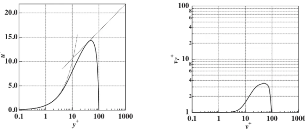
(2) 14 the oblique structure is tilted approximately 25 degree in the streamwise direction. Further lowering the Reynoıds number resulted in the limit state: at Re_{\tau}=45 , the angle of obıiqueness became approximately 45 degree. The mechanism of these oblique‐band formations at very low Reynolds numbers has not yet been eıucidated. At such a low Reynolds number, the spanwise wavelength (\lambda_{z}^{+}\sim 100) of the low‐speed streak structure near the wall is as large as the channel width (2d) . This leads to an imperfect scale separation of structures. Their nonlinear mutual interaction may affect on the growth of turbulence and on the global critical Reynolds number of the subcrtical transition which the wall‐bounded shear flow undergoes.. In this study, the maximum growth rate of the disturbance in the plane channel flow is computed,. although the attempt is as same as that is carried out by del Álamo and Jiménez (2006) and Pujals. et al. (2009), specialıy at a Reynolds number lower than the critical value based on the classical Orr‐. Sommerfeld equations. We attempt to eıucidate phenomena occurring in the channel flow field in such a low Reynoıds number based on the required method.. 2. Procedure. Computational method The three‐dimensional linear perturbation equation is described as follows;. \frac{\parti lu_{\lambda}^{\prime+}{\parti lt^{+} \frac{\parti l}{\parti l x_{j}^+}(\overline{u}_{i^+}u_{j}^\prime+} u_{i}^\prime+}\overline{u}_{j^ +})=-\frac{\parti lp^{\prime+}{\parti lx_{i}^+} \frac{\parti l}{\parti lx_ {j}^+}(\nu_{T}^{+}\frac{\parti lu_{i}^\prime+}{\parti lx_{j}^+}) In the equation, (\overline{u}_{?}^{+},\overline{p}^{+}) is the base flow and. .. (1). (u_{\dot{i} ^{\prime+}, p^{\prime+}) is the perturbation. The superscript. that non‐dimensionaıization is done on the viscous scaıe near the wall.. +. indicates. We assume that the flow is. homogeneous in the streamwise (x‐) and spanwise (z‐) directions. Pressure gradient of the base flow, \partial\overline{p}^{+}/\partial x^{+}, is set as 1. We consider the total eddy viscosity as a nonlinear effect, which is normalized by kinematic viscosity: \nu_{T}^{+}=\nu_{T}/\nu=1+\nu_{t}^{+} . The eddy viscosity \nu_{t}^{+} is given based on the formula proposed by Reynoıds and Tiederman (1967), as. f_{1} = 1- \eta^{2_{i} \int_{2}=1+2\eta^{2}, f_{3}=1-\exp(-\frac{(1-|\eta|)Re_ {\tau}}{A}) \nu_{t}^{+}. =. 0.. 5 \{1+(\frac{\kap a Re_{\tau}f_{1}f_{2}f_{3} {3})^{2}\}^{1/2}-0.5. The parameters in the expression,. A. and \kappa , are used as. .. ,. (2). and. A=26.5. \kappa=0.426 ,. respectively. The. average turbulent flow velocity distribution in the flow direction is. \frac{\parti l\overline{u}^{+} \parti l\eta}=-\frac{Re_{\tau^{\gam a}I {\nu_ {T}^{+}. .. (3). Here, \eta=y/d , the Reynolds number is defined as Re_{\tau}=u_{\tau}d/\nu . We calculate \overline{u}^{+} by Eq. (3) and the profile can be obtained explicitly, as given in Fig. 1. In this study, the maximum growth rate of perturbation is computed as. G_{\max}( \tau)=\Vert u^{f}(0)\Vert=1\max\frac{E(\tau)}{E(0)}=\max\lambda_{j}j. .. (4). The present computation program has been verified by comparison with laminar‐based solution (Butler and Farreıl, 1992) and that of turbulent one (Pujals et al., 2009). Here, the number of grid points in the wall‐normal direction is 129, and the time step is \triangle tu_{\tau}/d=0.001..

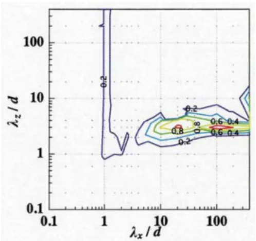
(3) 15. 0.1. 1. 10. 100. 1000. 0.1. 1. 10. y^{+} y^{+}. 100. 1000. Figure 1: Profiles of streamwise base flow \overline{u}^{+} (left), and the total eddy viscosity \nu_{T}^{+} (right).. Computational condition In accordance with the DNS result (Tsukahara and Ishida, 2014), we set the flow field at Re_{\tau}=50,. in which oblique bands of the localized turbulent region can be observed. At the vicinity of such low transitional Reynolds number, it has been observed that a turbulent spot which is locally turbulent occurs first and then the turbulent region gradually grows obliquely into a band‐shaped structure in downstream (Tsukahara and Ishida, 2014). Therefore, in the present study, we shall confirm the effect of the large‐ scale secondary flow in the spanwise direction which may excite the localized turbulence at the ıow Reynolds number.. We consider the spanwise velocity distribution as the base flow from DNS results. The distribution is modelled by the following equation for the sake of convenience.. \overline{w}^{+}(y/d)=\frac{w_{0}^{+} {36|\overline{u}^{+}| \exp(-y/\delta_{1} d)\cdot\sin(-2y/\delta_{2}d). .. (5). We apply w_{0}=1.0, \delta_{1}=0.4 and \delta_{2}=0.32 . The value of \overline{w} is 0 at the channel center and the maximum vaıue is \overline{w}^{+}=0.4 at approximately y/d=0.398 . The distribution is shown in Fig. 2.. 3. Results and discussion. The g]_{0}ba1 amplification rate, G_{globa1} , is obtained, which is the largest among the maximum growth rate of perturbation, G_{\max}(\tau) , of each target time, that \tau u_{\tau}/d is from 0.05 to 5.0, as given by the following equation:. G_{g{\imath} oba{\imath} = \max_{\tau}G_{\max}(\tau) .. (6). At first, if the flow condition is laminar without considering the nonlinear effect by eddy viscosity, G_{globa1} of any wavelength pair is less than 1.0. On the other hand, if the flow is turbulent, we observe a temporal energy amplification with specific wavelength pair, ( \lambda_{x} , A.). These results showed the same tendency as the results of the authors’ previous computations with \overline{w}=0 (Yakeno and Tsukahara, 2017). Secondly, in the case considering the spanwise velocity as the base flow, specific pairs of wavelength exhibits an increase in the temporal energy growth rate. Here, the difference of global amplification rate, Gglobal diff, between that with spanwise base flow, G_{g{\imath} oba{\imath}.w} , and that without the spanwise base velocity, G_{g}\iota_{obal} , is calculated as Gglobal,diff. =. Ggıobal. w-G_{g{\imath} oba{\imath}_{\dot{} }. and shown in Fig. 3. In the figure, the gray symbol of. +. (7). shows the pair of tested wavelengths (\lambda_{x}, \lambda_{z}) .. Among trials in this study, the peaks of G_{g}\iota_{obal,diff} are found at (\lambda_{x}, \lambda_{z})=(20,3) and (100, 3) for the.

(4) 16 early stage of transition, i.e., \tau u_{\tau}/d=1.5 . This indicates that the growth rate of the disturbance mode increases, which corresponds to the oblique direction when the span direction velocity is considered as the base flow.. In the future, we will investigate further details of the mechanism that the spanwise velocity around the turbulent flow spot enlarges the localized turbulent region obliquely, by increasing the trial wavelength, identifying the disturbance mode corresponding to the oblique direction, and confirming the Reynolds number dependency.. 1. \sim^{\aleph}\aprox (. 0.1. \overline{w}^{+} Figure 2: Profile of spanwise base flow w^{+}.. 1. 100. Figure 3: Contour of increase of the global amplifi‐ cation rates with spanwise base flow for each wave‐. length modes, G_{g}\iota_{obal_{:}} dif. 4. 10. \lambda_{l}ld. f.. Conclusion. We computed the most amplified non‐normal mode of transient growth for a plane channel flow at Re_{\tau}= 50 . It was found that the growth rate of the disturbance energy increased at specific pairs of wavelengths, when we consider the spanwise velocity around a turbulent spot/ band as a base flow. The present results imply that the spanwise secondary flow around a turbulent spotAband wouıd cause the transition in the oblique direction to form a large‐scale stripe pattern of localized turbulence.. Acknowledgement A.Y. acknowledges the support of the Grant‐in‐Aid for Scientific Research (B) (No. 15K21677 ). T.T. acknowledges the supports of the Grant‐in‐Aid for Scientific Research (A) (No. 16H06066 ) and on. Innovative Areas (No.. 16H00813 ). by Ministry of Education, Culture, Sports, Science and Technoıogy of. Japan.. References H. Abe, H. Kawamura, and Y. Matsuo. Direct numericaı simulation of a fully developed turbulent channel flow with respect to the Reynolds number dependence. Journal of Fluids Engineering, 123(2):382, 2001.. K. M. Butler and B. F. Farrell. Three‐dimensional optimal perturbations in viscous shear flow. Physics of Fluids, 4(8):1637-1650 , 1992..

(5) 17 J. C. del Álamo and J. Jiménez. Spectra of the very large anisotropic scales in turbulent channels. Physics of Fluids, 15(6):L41, 2003.. J. C. del Áıamo and J. Jiménez. Linear energy amplification in turbulent channels. Journal of Fluid Mechanics, 559:205, 2006.. W. Heisenberg. On stability and turbulence of fluid flows. 1951.. K. C. Kim and R. J. Adrian. Very large‐scale motion in the outer layer. Physics ofFluids, 11(2) :417-422, 1999.. L. D Landau. On the problem of turbulence. In Dokl. Akad. Nauk SSSR, 1944.. G. Pujaıs, M. Garcia‐Villalba, C. Cossu, and S. Depardon. A note on optimal transient growth in turbulent channel flows. Physics of Fluids, 21:015109, 2009.. S. C. Reddy and D. S. Henningson. Energy growth in viscous channel flows. Journal ofFluidMechanics, 6:209−238, ı993.. O. Reynolds. An experimental investigation of the circumstances which determine whether the motion of water shall be direct or sinuous, and of the law of resistance in parallel channels. Proceedings of the Royal Society of London, 35(224 ‐ 226):84-99 , 1883.. W. C. Reynolds and W. G. Tiederman. Stability of turbulent channel flow, with application to Malkus’s theory. Journal of Fluid Mechanics, 27(02):253-272 , mar 1967.. L. N. Trefethen, A. E. Trefethen, S. C. Reddy, and T. A. Driscoll. Hydrodynamic stability without eigenvalues. Science, 261:578−584, 1993.. T. Tsukahara and T. Ishida. The lower bound of subcritical transition in plane Poiseuille flow. In EU‐ ROMECH, Colloquium EC565, 2014.. T. Tsukahara, Y. Kawaguchi, H. Kawamura, N. Tillmark, and P. H. Alfredsson. Turbulence stripe in transitional channeı flow with/without system rotation. In D. S. Schlatter, P. & Henningson, editor, Proc. Seventh IUTAM Symp. on Laminar‐Turbulent Transition, pages. 421-426.. Springer, 2010.. T. Tsukahara, Y. Seki, H. Kawamura, and D. Tochio. DNS of turbulent channel flow at very low Reynolds numbers. In TSFP DIGITAL LIBRARY ONLINE. Begel House Inc., 2005.. A. Yakeno and T. Tsukahara. Linear transient growth of coherent structure in turbulent channel flow at low Reynolds number. In 10th lnternational Symposium on Turbulence and Shear Flow Phenomena (TSFP10), 2017..

(6)