Mathematical analysis to coupled oscillators system with a conservation law (Theory of Biomathematics and its Applications IV)

Mathematical

analysis

to

coupled

oscillators system

with

a

conservation

law

宮路

智行, 大西 勇

(T.Miyaji

and

I.Ohnishi)

広島大学大学院理学研究科数理分子生命理学専攻

Dept.

of Math.

and

Life

Sciences,

Graduate

School of Science, Hiroshima

University

1

lntroduction

We

are

interested in bifurcation structure of stationary solution for

a

3-component reaction-diffusion

systemwith

a

conservation law in the following:

$\{\begin{array}{l}\frac{\partial u}{\partial t}=\nabla\cdot(D_{u}\nabla u)+f(u, v)+\delta w\frac{\partial v}{\partial t}=\nabla\cdot(D_{v}\nabla v)+g(u,v)\frac{\partial w}{\partial t}=\Delta(D_{w}w)-f(u, v)-\delta w\end{array}$ (1.1)

where the functions $f(u,v)$ _and $g(u, v)$

are

chosenin such forms that the local oscillator

$\frac{du}{dt}=f(u, v)$, $\frac{dv}{dt}=g(u,v)$ (1.2)

can

undergo thesupercritical Hopfbifurcation. Obviously, the totalamountof$u+w$ is conserved under

homogeneous Neumann (no-flux) boundary conditionand

some

natural andappropriate conditions.

In [4], they proposethissystem tounderstandtheperiodicoscillationofthe body oftheplasmodium of

thetrueslimemold: Physarum polycephalum. Infact,thesystemdescribesthetime-evolution of$(u, v, w)$,

which may obtain

some

spatio-temporal oscillation

so

lutions. We explain the mechanism heuristically

in the following: We note that if$w$ does not exist, then thesystem is

a

coupledoscillatorssystem with

diffusion coupling. This system has temporally oscillation solutions, but does not have any spatlally

structural solution. It is sure that this system is not appropriate for the model system just

as

it is,

but the body of the plasmodium of Physarum polycephalum can be separated in the two parts;

one

is

a

sponge part, the other is

a

tubular part. The characteristic property is that the diffusion rates

are

quite different between the former part and the latter part. Namely, the diffusion coefficient of tubular

part is quite larger than the

one

ofsponge part. This is why they have considered the

new

variable $w$,

which

means

thetubular part and the diffusion coefficient of$w$ is muchlarger than those

of

$u,v$

.

Here

$u$ standsfor the

sponge

part,and$v$represents the effect of the other ingredients, which let the desirable

oscillations

occur.

Our objective is that

we

understand how many structural varieties this system has

from theviewpointofbifurcation ofstationarysolutions. Note that $D_{u},$$D_{v}\ll D_{w}$ should holdinorder

todescribe the behavior of plasmodium.

In biological experiment, for example, ifyou watch

a

circularplasmodium propagating

on a

flat ager

surface, you

can

observe

an

anti-phase oscillation between the peripheral region and the

rear

of the

assumptionthat$D_{u}$ and$\delta$depend

on

the space variable andreproducetheperipheralphaseinversion

by numericalsimulation. This is very interesting for

us

too, and

we

have noticed thattheoriginal system

withconstant coefficients is also

a

mathematically attractiveobject. This is becausethissystem has

the

mass

conservation law, sothat a kindof “degree offreedom” ofsolutionsmaybe less than the usual

3-component system, which undergoes

wave

_{bifurcations.}

Therefore, in this study,

we

assume

that all

the coefficients

are

constant. We investigate behaviorof solution orbit of thesystem

near

the Hopf

bifurcation point of theorigin. Especially, wave instability is our interest. The

wave

instability breaks

both spatial and temporalsymmetries of

a

$homogen\infty us$state while the (uniform) Hopfbifurcation does

only temporal symmetry $[3, 5]$

.

In [3],itissaidthatthe

wave

instability

occurs

when

a

homogeneousstate

becomes unstable by

a

pair of purely imaginary eigenvalues with spatially non-uniformeigenfunctions.

We consider thesystem

on an

interval $\Omega=[0,1]$ withhomogeneousNeumannboundarycondition and

supposethat $D_{u}=D_{v}=\epsilon,$$D_{w}=1$

.

We adopt the$\lambda-\omega$system

as

asimplelocal oscillator. Therefore

we

study the following equations:

$\{\begin{array}{l}\frac{\partial u}{\partial t}=\epsilon\frac{\partial^{2}u}{\partial x^{2}}+\lambda u-\omega v+\delta w-u(u^{2}+v^{2})\frac{\partial v}{\partial t}=\epsilon\frac{\partial^{2}v}{\partial x^{2}}+wu+\lambda v-v(u^{2}+v^{2})\frac{\partial w}{\partial t}=\frac{\partial^{2}w}{\partial x^{2}}-\lambda u+\omega v-\delta w+u(u^{2}+v^{2})\end{array}$ (1.3)

We

can

prove mathematically rigorouslythatthe

wave

instability

can

occur

undernatural and

appro-priateconditions for this system. Wewill state themain statement of

our

theorem in the next section.

Moreover, in \S 3, we will show

some

graphs and figures obtained by numerical simulation in which

we

observe the Hopf critIcal points’ behavior foreach Fourier mode and observe the behavior of solutions

near

the bifurcation points at which

rwo

Fourier modes

are

made unstable at the

same

time. We

espe-cially notice that thissystem has

a

preferableclustersize ofsynchronizationofoscillations,which tends

to smaller and smalleras$\epsilon$goes to$0$

.

It may be interestingthat, ifthe effect bywhich the synchronized

oscillation

occurs

istoo much, then the synchronized cluster is vanishingand akind ofhomogenization

happens.

2

The linearized eigenvalue

problem

Theequations (1.3)can be written in matrix form

as

follows:

$\frac{\partial U}{\partial t}=(D\frac{\partial^{2}}{\partial x^{2}}+\Lambda)U+F(U)$, (2.1)

where$U=(u,v,w)$,

$D=(\begin{array}{lll}\epsilon 0 00 \epsilon 00 0 l\end{array})$ , A$=(\begin{array}{lll}\lambda -\omega \delta\omega \lambda 0-\lambda \omega -\delta\end{array})F(u)=(^{-u(u^{2}+v^{2}}-uv((u^{2}u^{2}++v^{2}v^{2})\})$

.

Remark 1. It is not necessary

_for

the resultsin this section that$\Omega$ is an interval. It is allowed$\Omega$ to be

n-dimensional bounded domain

_for

$n\geq 1$

.

Westudy the linearized system:

where $U=(u, v, w)$

.

Now we recall the eigenvalue problem of Laplacian with homogeneous Neumann

boundary condition [1].

$\{\begin{array}{ll}\Delta\psi_{n}=- \psi_{n},\frac{\partial\psi_{n}}{\partial\nu}=0 on \partial\Omega,\end{array}$ (2.3)

where$0=k_{0}^{2}<k_{1}^{2}\leq k_{2}^{2}\ldots$

.

If$\Omega=[0,1]$, then

we

obtain $k_{n}=n\pi$

.

For any integer $n$, the equations (2.2) admits solutions of the form $U_{n}(x, t)=V_{n}e^{\mu_{n}}{}^{t}\psi_{n}(x)$, where

$V_{n}\in \mathbb{R}^{3}$

.

Bysubstitution, we have the eigenvalue problem

$L_{n}V_{\mathfrak{n}}=\mu_{n}V_{n}$, (2.4)

wherethe matrix$L_{\mathfrak{n}}=\Lambda-k_{n}^{2}D$ is given by

$L_{n}=(\omega$ $\lambda-\epsilon k_{n}^{2}-\omega w$ $-\delta\delta-k_{n}^{2}0$

).

(25)

It is obvious that theeigenvaluesof$L_{0}=\Lambda$is identical to that of the local oscillator:

$\mu_{0}=0$, $\frac{1}{2}(2\lambda-\delta\pm\sqrt{\delta^{2}-4\omega^{2}})$

.

(26)

Next,

_we

consider the

case

of $n\neq 0$

.

The characteristic polynomial $\varphi_{n}$ of $L_{n}$ is cubic. It is not

impossible to express the solutions of$\varphi_{n}(\mu)=0$ explicitly, but it isnotsuitable for bifurcation $analy_{8}is$

.

So

we

take

a

qualitative approach. We give

a

sufficientcondition for the existence of a pair ofcomplex

conjugate eigenvalues of$L_{n}$ and its realpart becomespositive for some $n$

.

Theorem 1. Let$\lambda,\omega,$$\delta>0$ and$0<\epsilon<1$

.

If

thefollowing

four

inequalities hold

for

an integer$n$, then

$L_{n}$ has

a

negative eigenvatue and apair

of

complex conjugate eigenvalues:

$\lambda+\omega<\delta+k_{n}^{2}$ (2.7)

$2w<(1-\epsilon)k_{n}^{2}$ (2.8)

$2\lambda-\delta+2(1-\epsilon)k_{n}^{2}>0$ (2.9)

$\sqrt{\frac{\delta\lambda\{\delta+\lambda+(1-\epsilon)k_{n}^{2}\}}{2\lambda-\delta+2(1-\epsilon)k_{n}^{2}}}<\omega$ (2.10)

nnhermooe, under the above assumptions,

_if

$\epsilon\dot{u}$ sufciently small, then $L_{n}$ has a pair

of

complex conjugate eigenvalues with positivereal part.

Toprovethistheorem, we applyGershgorin’s$th\infty rem$(see [2] for detailof thetheorem). $Gershgorin’ 8$

theoremgives

us

arough estimate of the distribution ofeigenvaluesofmatrix

on

complex plane. If (2.7)

and (2.8) are satisfied, then $L_{n}$ has at least one negative eigenvalue. Thenwehave only toconsider the

shape of the graph of$\varphi_{n}(\mu)$, andfurthermorecalculationsfor$\varphi_{n}(\mu)$, in fact,giveus desiredinformations

about the arrangement ofthe roots of $\varphi_{n}(\mu)=0$

.

In details of the proof, please refer

our

forthcoming

paper in the

near

future.

Remark

2.

_If

theinequalities hold

_for

$n=1$, then $L_{n}$ has

a

negative eigenvalue and

a

pair

of

complex

conjugate eigenvalues

_for

$n\geq 1$

.

Especially, it should be noted that even

if

the real $p$art

of

O-mode

eigenvalue is negative $(2\lambda<\delta)$, then that

of

n-mode

can

be positive

for

some

$n\geq 1$

.

This implies that

the

wave

instability

occurs

mathematically rigorously.

Remark 3.

If

$D_{u}=D_{v}=D_{w}=d>0$, the problem is very easy. The eigenvatues

of

$L_{n}$ are given by

$\mu_{n}=-dk_{n}^{2}$, $\frac{1}{2}(2\lambda-\delta-2dk_{n}^{2}\pm\sqrt{\delta^{2}-4w^{2}})$

.

According to the monotonicity

_of

the eigenvalues

of

Laplacian, O-mode is the most unstable. Thenfore,

3

Numerical

simulations

In this section, we briefly _{show the results obtained by numerical simulation. The} system (1.3) with

zero-flux boundary condition

was

solved numerically in

one

spatial dimension using

a

explicit finite

difference method. To calculate the eigenvalues of each matrix$L_{n}$,

we

employed the QR method.

We have already known that the eigenvalues of$L_{n}$ areone negative and a pair of complex $\infty njugate$

.

Therefore

we

focus

on

the real parts ofthe complex eigenvalues$\mu_{\mathfrak{n}}$ to study the bifurcation structure.

Figure 1 shows eachHopfbifurcation

curve

$({\rm Re}\mu_{n}=0)$forcorrespondingFourier modeintheparameter

space $(\delta, \lambda)$ for

some

fixed $\epsilon$

.

Here $\epsilon$ is the diffusion coefficient of

$u$ and $v$

.

Small $\epsilon$ leads to spatially

non-uniform Hopf bifurcation, that is,

wave

instability. If$\epsilon$ is chosensmaller, then the higher Fourier

mode becomes unstable

as

the first bifurcation. Hence it

can

be said that fast diffusion of $w$ plays

an

important role for the emergenceof the

wave

instability in (1.3). As shown in Figure 1, each ofHopf

bifurcation

curves can

intersect. These

intersections

imply

wave-wave

interactions.

Figure 2 shows the behavior of themost unstable modenumber

as

$earrow 0$

.

Theparameters

are

chosen

so

that $R\epsilon\mu_{0}=0$

.

At $\epsilon=1$,O-modeeigenvalue is themost unstable. However, the most unstable mode

numberchanges successively

as

$\epsilon$ approaches to

zero.

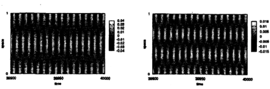
Figure 3 shows stable standing wavesolutions. The 2-mode$8tanding$ wave solution is very similar to

peripheral phaseinversion behavior ofplasmodium. Ofcourse, standing

waves

withdifferent wave-length

can be observed for corresponding parameters. Furthermore, spatiotemporal patterns arising from the

interaction between

wave

instabilitiesof different modes

can

beobserved.

何 $R-$ 何 $Ra$

Fig. 1 Hopfbifurcation curvesin$(\delta,\lambda)$-plane. Parameter: _{$\epsilon=0.01(left),\epsilon=0.\alpha)01(right)$}

.

Flg. 2 The most unstable mode number increases as $\epsilonarrow 0.The$ parameters are $(\lambda,w,\delta)=$

$(0.5,1,1).The$ horizontal line indicates $\log_{10}\epsilon$ and the vertical line does the mode number which

Fig. 3 Stable standing wave solutions. The left is 2-mode oscillation for $(\lambda,w, \delta,\epsilon)$ $=$

(0.005,1,1, 0.001). The right is 3-mode oscillation for$(\lambda,w,\delta,e)=(0.0004,1,1, 0.000003)$

time

Fig. 4 Modeinteractionbetween l-mode and2-mode.

4

Discussion,

Conclusion,

and

Future

works

In thesystem (1.3),the

wave

instabilityplaysacentraland crucial role forpattemformation. It turned

out the pattem like peripheral phase inversionto be naturally

included

in the system. In addition, the

system can exhibit many other spatiotemporalstructures. Therefore, from the viewpoint of

our

study,

we

can

interpret the work in [4]

as

follows: To understand the behavior of the plasmodium system

mathematically, they crushed the structures in which the solution did not behave like the plasmodium

system of Physarum polycephalum by considering spatially dependence of coefficients naturally. AI

a

result, theysucceeded to construct the mathematical model which

was

betterto reproducebehavior of

the plasmodium systemcleverly.

In this study, $D_{u}=D_{v}$ is assumed. If $D_{u}\neq D_{v}$, the Turing instability might be caused. In [5],

they study the pattern formation arising from the interaction between Turing and

wave

instability in

3-component oscillatory reaction diffusionsystem. Their system does not satisfy any conservation law.

In thefuture,wewould like to consider that how different the structure ofbifurcationsis? On the other

hand, thehomogenizationof thesynchronizedoscillation clustersize, whichhas been already mentioned

in \S 1, is anothermathematically interesting problem. We try tomake this be amathematical result.

References

[1] Courant, R. andHilbert,D.: MethodsofMathematicalPhysics,IntersciencePublishers, NewYork(1953).

[2] Ftanklin, J.N.:Matrix$Th\infty ry$, PrenticeHall,Englewood CliffU, NJ (1968).

[3] Ogawa, T.: Degenerate Hopf instability in $\propto cillatory$ reaction-diffusion equations, DCDS Supplements,

Specialvolume (2007), pp.784-793.

[4] Tero, A., Kobayashi, R. and Nakagaki, T.: A coupled-oscillator model with a $con\epsilon enation$ law for the rhythmicamoeboid$movement_{8}$of plasmodialslime$mold_{8}$, Physica$D$ 205 (2005), pp.125-135.

$|5]$ Yang, L., Dolnik, M., Zhabotinsky, A. M., and Epstein, I. R.: Pattern formation arisingfrom interactions