Evaluation of Wind Speed Potential Using Correlation Coefficient Model in Medan, North Sumatra, Indonesia

第 56 卷 第 1 期

2021 年 2 月

JOURNAL OF SOUTHWEST JIAOTONG UNIVERSITY

Vol. 56 No. 1

Feb. 2021

ISSN: 0258-2724 DOI：10.35741/issn.0258-2724.56.1.6

Research article

Electrical and Electronic Engineering

E

VALUATION OF

W

IND

S

PEED

P

OTENTIAL

U

SING

C

ORRELATION

C

OEFFICIENT

M

ODEL IN

M

EDAN

,

N

ORTH

S

UMATRA

,

I

NDONESIA

基于相关系数模型的印尼北部苏门答腊棉兰风速潜力评估

Suwarno

Department of Electrical Engineering, Muhammadiyah University of North Sumatra Medan, North Sumatra, Indonesia, [email protected]

Received: November 18, 2020 ▪ Review: December 23, 2020 ▪ Accepted: January 20, 2021:

This article is an open-access article distributed under the terms and conditions of the Creative Commons Attribution License (http://creativecommons.org/licenses/by/4.0)

Abstract

Medan is the capital city of North Sumatra Province, consisting of various tribes and a dense population that requires a large amount of electrical power. Energy demand continues to increase along with population and business growth, so that additional energy sources are needed; one of which is wind. An evaluation of the potential of wind energy sources is needed to determine the feasability of its use as an environmentally-friendly, renewable energy source without emissions.This paper aims to evaluate the potential wind speed in the city of Medan using the correlation coefficient (R2) model. The four application models proposed for the probability density function used are Normal Distribution, Lognormal, Weibull 2-parameters and Weibull 3-parameters. The analysis results show that the four models used are all potentially feasible options that can be used to evaluate the potential sources of wind energy in Medan. The potential of these models for use, ranked from most to least, are the Weibull 3-parameter Model, followed by the Lognormal, Normal Distribution and Weibull2-3-parameter. In addition to the analysis, the results of the Normal, Lognormal and Weibull Distribution tests are also presented.

Keywords: Wind Speed, Probability Density Function, Correlation Coefficient

摘要 棉兰是北苏门答腊省的省会城市，由各种部落组成，人口众多，需要大量电力。能源需求随 着人口和企业的增长而持续增长，因此需要更多的能源；风之一。需要评估风能的潜力，以确定 将其用作无排放的环保，可再生能源的可行性。本文旨在利用相关系数（R2）评估棉兰市的潜在 风速）模型。针对所使用的概率密度函数建议的四个应用模型是正态分布，对数正态，威布尔 2 参数和威布尔 3 参数。分析结果表明，使用的四个模型都是可以用来评估棉兰潜在风能来源的潜 在可行方案。这些模型的使用潜力（从最高到最低）依次是威布尔 3 参数模型，其次是对数正态 分布，正态分布和威布尔 2 参数。除了分析之外，还提供了正态，对数正态和威布尔分布检验的

结果。

关键词:风速，概率密度函数，相关系数

I. I

NTRODUCTION

Renewable energy sources began to grow in the early seventies due to the fossil energy crisis that hit the energy market at that time [1]. As the global demand for energy is growing rapidly, it is time to look for new and renewable energy sources to replace the dwindling fossil fuel supply [2], [3]. One alternative and renewable energy option is wind energy. To determine the potential of wind energy, an evaluation of the probability density function (PDF) is performed. The choice of PDF is very important in the evaluation of wind energy, because wind power is calculated as an explicit function of wind speed distribution parameters. Evaluation of the wind speed probability density function is performed using the four proposed models using the coefficient of determination (R2) in this study, and the data feasibility test uses the Kolmogorov–Smirnov test (K-S).

II. L

ITERATURE

R

EVIEW

The Weibull2-parameter distribution and the Rayleigh distribution are most commonly used in wind speed data analysis, especially for studies related to wind energy estimation [4], [5], [6], [7], [8]. The 2-parameter Weibull distribution is the most widely used distribution for wind speed characterization, and has a number of advantages for this purpose [9]. The Rayleigh distribution, the one-parameter distribution, and the two-parameter Weibull distribution are most often used in studies related to wind speed analysis [10], [11].

The 3-parameter Weibull model with

additional location parameters has been used in studies by Stewart and Essenwanger [12], and Tuller and Brett [9]. Generally, this model is

more suited to the Weibull3-parameter

distribution than the usual Weibull 2-parameter distribution. The model provides a better fit for wind speed data than some of the other distributions. Recently, other standard PDFs have been used to characterize wind speed distribution [13], [14], [15], [16]. The general model used was a mix of Weibull2-parameters with a single-cut normal distribution from the bottom with Weibull2-parameter distribution. The mixed model was found to be suitable for the bimodal wind regime [13].

This approach was adopted by Zhang et al. [17] in a multivariate framework, since the minimum threshold wind speed was required to be recorded by the anemometer and a wind speed of zero occurred frequently. However, for many distributions, including the Weibull2-parameter, a wind speed of zero was not taken into account correctly because the CDF of this distribution provided zero probability of observing a wind speed of zero of a given variable X. Of the various PDFs that show relative levels of fit with wind-speed data as samples, some statistics were used in studies related to wind-speed analysis. The coefficient of determination (R2) was most often used [8], [18], [19], [20], but chi-square test results [11], [21], [22], [23], Kolmogorov– Smirnov (KS) test results [9], [22], [24], [25], and root mean square error (RMSE) were also used [11], [24], [26], [27]. In most studies, a visual assessment of the attached PDF overlaid on the wind-speed data histogram was also performed [28], [29], [30]. R2 and RMSE were applied either to the theoretical cumulative probability, to the empirical cumulative probability (PP plot) [13], [31], [32], [33], or to the theoretical wind speed of the observed wind-speed quantile (QQ plot) [8], [11], [17]. These statistics were also sometimes calculated with wind-speed data in a frequency histogram [13], [31].

In addition to the analyses conducted on wind-speed distribution, several authors also evaluated the suitability of PDF in matching the power distribution obtained from the sample wind speed and in predicting energy output [8], [24], [27], [34]. In this case, PDF was first attached to the wind-speed data. Then, the theoretical power-density distribution was derived from the PDF adjusted for wind speed. Finally, the measure of relative level of fit was calculated using the theoretical wind-power density distribution and the estimated power distribution from the wind-speed sample. Analysis was performed on the cube of wind speed compared to wind power [4], [31].

III. D

ATA

Data on the climate of thecity of Medan was obtained from the Meteorological, Climatological, and Geophysical Agency (MCGA), which provides observations on average wind speed

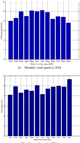
over a recorded 30-minute range; the location of the observations is shown in Figure 1.The monthly wind-speed characteristics of Medan are shown in Figure 2. We analyzed the average wind-speed data of three years, starting from 2017 until 2019. The wind-speed characteristics of those three years were of the same type as shown in Figure 3. The set of data obtained from these observations of average monthly wind speed, as well as short-term wind-speed measurements, were obtained from Sampali station and are available online.

Figure 1. Location of wind speed observation in Medan city

a) Monthly wind speed in 2017

b) Monthly wind speed in 2018

c)Monthly wind speed in 2019

Figure 2. Characteristics of wind speed in Medan city

IV. M

ETHODOLOGY

A. Wind-Speed Distribution

The city of Medan is located in the equatorial region. It has a hot summer with temperatures around 23–33°C and humidity around 63%–82%, as shown in Figure 3. Medan makes up 26,510 hectares (265.10 km²), or 3.6%, of the total area of North Sumatra. Thus, compared to other cities/districts, Medan has a relatively small area with a relatively large population. Geographically, Medan is located at 3°30'-3°43” N latitude and 98°35'-98°44” E longitude. For this reason, the topography of Medan City tends to slope to the north at an altitude of 2.5–37.5 meters above sea level. It has a tropical rainforest climate with an indistinct dry season [33]. The city has wetter and drier months, with the driest (February) experiencing an average of about one-third as much precipitation as seen in the wettest month (October). The temperature in Medan averages around 27°C throughout the year. Wind speeds

Jan Feb Mar Apr May Jun Jul Aug Sep Oct Nov Dec

0 1 2 3 4 5 6 W in d s p e e d ( m /s )

are generally below 8 m/s for most of the year. Strong winds with an average speed exceeding 10 m/s overland occur due to weather systems, such as active surface troughs or storm lines.

Figure 3. Average weather in Medan city B. Probability Distribution

The probability distribution describes a set of variants as a replacement frequency. The cumulative probability is the probability of a random variable being equal to or less than a certain value. The probability density function (PDF) is the probability value of each event, while the cumulative density function (CDF) adds up the probability value to a certain event. The probability of occurrence of wind speed (v), parameters k, and c is fully positive. The form factor is the wide distribution of wind speed identification and determines the peak wind distribution in each region [35]. The scale factor is the identification of the abscissa scale of the wind distribution and the condition of most of the wind potentials in a location [20]. The identification of the distribution is more suitable using the Weibull three-parameter distribution (W3) when compared to W2 [36]. Wind speed can be modeled with the Weibull distribution and truncated normal distribution [37]. Using the distribution of W2, W3, generalized gamma, and Burr 4 parameters to describe the wind speed profile in Antakya, Turkey [38].

The determination of the PDF and CDF values is given as follows:

PDF Weibull distribution is k k x x k x f              







exp ) ( 1 (1) PDF Normal Distribution is      _   ₂ 2 2 ) ( exp 2 1 ) (









x x f (2) PDF log-normal distribution is      _  









2 ) (log exp 2 1 ) ( 2 x x x f (3)

Statistically based method of calculating multiple parameters from any data distribution, assuming that the parameter value giving the maximum value of the possible function is the most likely value. According to this method, the c and k parameters are calculated with the total data points indicated by N [39], [40].

 

 

1 1 1 1 1 ln ln              







N v v v v k N i i N i k N i i k i (4) k N i k i

v

N

c

1 1

1













_ (5)

Wind speed data expressed by the MLM in the form of scale and shape parameters [24], [39], [41].

 

 

1 1 1 1 1 ) 0 ( ) ( ln ) ( ) ( ln               







v f v f v v f v v f v v k N i i i N i i k N i i i k i (6) k i N i k i i f v f c 1 1 1         





 (7) C. Determination Coefficient (R2)

The coefficient of determination (R2) is the ratio of the Regression Sum of Squares (SSR) to the Total Sum of Squares (SST), which gives little about regression variation. The SSR ratio to SST measures the proportion of the variable in Y, which is explained by the independent variable X in the regression model. The coefficient of determination (R2) is stated by:

SST SSR R2  (8) where:



_  











 



n i

y

i

y

SSR

1 2



          n i yi y SST ₁ 2



i

y is estimated by the regression line i

y

is the value in a sample



y is the mean value of a sample

V. R

ESULTS AND

D

ISCUSSION

For the distribution test model in Figures 4, 5, and 6 for each model, the better fit for the three distribution test models is normal, log normal,

and Weibull distribution. The possible

comparison distribution method with the

correlation coefficient (R2) is shown in Figures 7, 8, 9, and10, respectively, for the normal distribution, lognormal distribution, Weibull 2 parameters, and Weibull 3 parameters.

Monthly wind speed data Figure 4. Normal distribution

Monthly wind speed data Figure 5. Lognormal distribution

Monthly wind speed data Figure 6. Weibull distribution

Based on the results of the wind speed distribution test given in Figures 4, 5, and 6 with the three distribution models for 2017–2019, it gives the same model, which tends to the right, to fit the expected distribution test model. The probability density function (PDF) for the four proposed models is shown in Figure 7 for normal distribution, Figure 8 for lognormal distribution, Figure 9 for Weibull distribution two parameters, and Figure 10 for Weibull distribution three parameters.

Wind speed (m/s) Figure 7. Normal distribution

Wind speed (m/s) Figure 8. Lognormal distribution

Wind speed (m/s) Figure 9. Weibull 2 parameters

Wind speed (m/s) Figure 10. Weibull 3 parameters

Based on the results of the distribution comparison with correlation coefficient (R2) test shown in Figures 7, 8, 9, and 10, each Normal distribution model, Lognormal, Weibull two parameters, and Weibull three parameters for 2017–2019 provide correlation coefficient values, as shown in Table 1 for each of the proposed models. The test results of four models, namely

Weibull two parameters, Weibull three

parameters, Normal, and Lognormal distribution, are shown in Table 1.

Table 1.

The test results of Weibull two parameters, Weibull three parameters, Normal, and Lognormal distribution No Distribution function

b

t

0

T

 x s _Median 2

R

1. Weibull 2-parameter 2.633 - 11.92504 - - - 0.8530 Weibull 3-parameter 0.99 5.232537 10.74797 - - - 0.9981 2. Normal - - - 10.579±1.505 5.1936 - 0.8790 3. Lognormal - - - - 1.5561 9.6572±0.056 0.9580

In addition to evaluating the wind speed distribution test, the results of the monthly goodness-of-fit test using Kolmogorov-Smirnov (K-S) for three years were also given, as shown in Table 2.

Table 2.

The test statistic of data for 2017-2019

Monthly 2017 2018 2019 K-S K-S K-S January 0.957 0.957 0.650 February 0.697 0.760 0.587 Mart 0.616 0.591 1.065 April 0.966 1.101 0.942 May 0.542 0.640 0.718 Juni 0.919 0.884 0.668 July 0.950 0.921 0.772 August 0.831 0.860 1.151 September 0.581 0.612 0.693 October 0.757 0.887 0.720 November 0.755 0.878 0.622 December 0.832 0.851 0.878

Based on the test results in Table 2, the K-S test for each month and year shows a value greater than 0.05 (95%), which provides that the research data were normally distributed and deserves to be done as the data of this study.

VI. C

ONCLUSION

The results of the analysis that have been carried out with the four distribution models proposed using the correlation coefficient (R2). In general, the four models provide the expected results. However, the best results are obtained

with the 3-parameter Weibull distribution model, which is then followed by lognormal, normal distribution, and Weibull 2 parameters. This is shown by the magnitude of the correlation coefficient, which is close to one (1) the best.

A

CKNOWLEDGMENT

The author would like to thank the Chief Editor for providing the opportunity to fill in this journal. The author also hopes that this manuscript can is accepted and published.

R

EFERENCES

[1]

JOHANSSON, T.B., BURNHAM, L.,

KELLY,

H.,

REDDY,

A.K.N.,

and

WILLIAMS, R. (1993) Renewable Energy:

Source for Fuels and Electricity. Washington,

District of Columbia: Island Press.

[2]

NANSAIOR, A., PATANOTHAI,A.,

and RAMBO, A.T. (2013) The sustainability

of biomass energy acquisition by households

in urbanizing communities in Notheast

Thailand. Biomass and Bioenergy, 52, pp.

113-121.

[3]

ZOU, C., ZHAO, Q., ZHANG, G.,

and XIONG, B. (2016) Energy revolution:

From a fossil energy era to a new energy era.

Natural Gas Industry B, 3 (1), pp. 1-11.

[4]

HENNESSEY, J.P.Jr. (1977) Some

aspects of wind power statistics. Journal of

Applied Meteorology, 16 (2), pp. 119-128.

[5]

NFAOUI, H., BURET, J., and

SAYIGH,

A.A.M.

(1998)

Wind

characteristics and wind energy potential in

Morocco. Solar Energy, 63 (1), pp. 51-60.

[6]

ŞAHIN, A.Z. and AKSAKAL, A.

(1998) Wind power energy potential at the

northeastern

region

of

Saudi

Arabia.

Renewable Energy, 14 (1-4), pp. 435-440.

[7]

PETKOVIĆ, D., SHAMSHIRBAND,

S., ANUAR, N.B., SABOOHI, H., WAHAB,

A.W.A., PROTIĆ, M., ZALNEZHAD, E.,

and MIRHASHEMI, S.M.A. (2014) An

appraisal

of

wind

speed

distribution

prediction by soft computing methodologies:

a comparative study. Energy Conversion and

Management, 84, pp. 133-139.

[8]

CELIK, A.N. (2004) A statistical

analysis of wind power density based on the

Weibull and Rayleigh models at the southern

region of Turkey. Renewable Energy, 29 (4),

pp. 593-604.

[9]

TULLER, S.E. and BRETT, A.C.

(1985) The goodness of fit of the Weibull

and Rayleigh distributions to the distributions

of observed wind speeds in a topographically

diverse area. Journal of Climatology, 5 (1),

pp. 79-94.

[10]

CELIK,

A.N.

(2003)

Weibull

representative compressed wind speed data

for energy and performance calculations of

wind energy systems. Energy Conversion

and Management, 44 (19), pp. 3057-3072.

[11]

AKPINAR, E.K. and AKPINAR, S.

(2004) Statistical analysis of wind energy

potential on the basis of the Weibull and

Rayleigh distributions for Agin-Elazig,

Turkey. Proceedings of the Institution of

Mechanical Engineers, Part A: Journal of

Power and Energy, 218 (8), pp. 557-565.

[12]

STEWART,

D.A.

and

ESSENWANGER, O.M. (1978) Frequency

distribution of wind speed near the surface.

Journal of Applied Meteorology, 17 (11), pp.

1633-1642.

[13]

CARTA, J.A. and RAMIREZ, P.

(2007) Analysis of two-component mixture

Weibull statistics for estimation of wind

speed distributions. Renewable Energy, 32

(3), pp. 518-531.

[14]

WU, D., HAN, Z., LIU, Z., and

ZHANG, H. (2019) Study on configuration

optimization

and

economic

feasibility

analysis for combined cooling, heating and

power system. Energy Conversion and

Management, 190, pp. 91-104.

[15]

BHATTACHARYA,

P.

and

BHATTACHARJEE, R. (2009) A study on

Weibull distribution for estimating the

parameters. Wind Engineering, 33 (5), pp.

469-476.

[16]

OWUSU, P.A. and

ASUMADU-SARKODIE, S. (2016) A review of

renewable energy sources, sustainability

issues and climate change mitigation. Cogent

Engineering, 3 (1), 1167990.

[17]

ZHANG, H., YU, Y.-J., and LIU,

Z.-Y. (2014) Study on the Maximum Entropy

Principle applied to the annual wind speed

probability distribution: A case study for

observations of intertidal zone anemometer

towers of Rudong in East China Sea. Applied

Energy, 114, pp. 931-938.

[18]

GARCIA,

A.,

TORRES,

J.L.,

PRIETO, E., and DE FRANCISCO, A.

(1998) Fitting wind speed distributions: a

case study. Solar Energy, 62 (2), pp. 139-144.

[19]

AKPINAR, S. and AKPINAR, E.K.

(2009) Estimation of wind energy potential

using finite mixture distribution models.

Energy Conversion and Management, 50 (4),

pp. 877-884.

[20] SHU, Z.R., LI, Q.S., and CHAN, P.W.

(2015)

Statistical

analysis

of

wind

characteristics and wind energy potential in

Hong Kong.

Energy Conversion and

Management, 101, pp. 644-657.

[21]

VAN DER AUWERA, L., DE

MEYER, F., and MALET, L.M. (1980) The

use of the Weibull three-parameter model for

estimating mean wind power densities.

Journal of Applied Meteorology, 19 (7), pp.

819-825.

[22]

DORVLO, A.S.S. (2002) Estimating

wind speed distribution. Energy Conversion

and Management, 43 (17), pp. 2311-2318.

[23]

CHANG, T.P. (2011) Performance

comparison of six numerical methods in

estimating Weibull parameters for wind

energy application. Applied Energy, 88 (1),

pp. 272-282.

[24]

CHANG, T.P. (2011) Estimation of

wind energy potential using different

probability density functions. Applied Energy,

88 (5), pp. 1848-1856.

[25]

USTA, I. (2016) An innovative

estimation

method

regarding

Weibull

parameters for wind energy applications.

Energy, 106, pp. 301-314.

[26] SUWARNO, C., ADI, S., and DAUD,

I. (2012) The Potential Wind To Electrical

Energy Using A Linear Regression Method

in Medan City. In: Prosiding Seminar

Nasional

2012

“Teknik Elektro Dan

Informatika

Dalam

Pengembangan

Teknologi Berkelanjutan”, Mataram, July

2012, pp. 183-188.

[27] SEGURO, J.V. and LAMBERT, T.W.

(2000) Modern estimation of the parameters

of the Weibull wind speed distribution for

wind energy analysis. Journal of Wind

Engineering & Industrial Aerodynamics, 85

(1), pp. 75-84.

[28]

WANG, J., HU, J., and MA, K.

(2016) Wind speed probability distribution

estimation and wind energy assessment.

Renewable and Sustainable Energy Reviews,

60, pp. 881-899.

[29]

SUWARNO, S. and ROHANA, R.

(2017)

Comparison

model

hargreaves,

annandale and new model for estimation of

solar

radiation

in

Perlis,

Malaysia.

Indonesian Journal of Electrical Engineering

and Computer Science, 6 (2), pp. 286-293.

[30]

TSANG, A. and JARDINE, A. (1993)

Estimators

of

2-Parameter

Weibull

Distributions from Incomplete Data with

Residual Lifetimes. IEEE Transactions on

Reliability, 42 (2), pp. 291-298.

[31]

CARTA, J.A., RAMIREZ, P., and

VELAZQUEZ, S. (2009) A review of wind

speed probability distributions used in wind

energy analysis: Case studies in the Canary

Islands. Renewable & Sustainable Energy

Reviews, 13 (5), pp. 933-955.

[32] SUMAIR, M., AIZED, T., GARDEZI,

S.A.R., UR REHMAN, S.U., and REHMAN,

S.M.S. (2020) A novel method developed to

estimate Weibull parameters. Energy Reports,

6, pp. 1715-1733.

[33]

ALI, S.M., SHABAN, A.H., and

RESEN,

A.K.

(2014)

Wind

Power

Estimation for Al-Hay District (Eastern

South of Iraq). Iraqi Journal of Science, 55

(4B), pp. 1997-2004.

[34]

MOHAMMED,

D.,

MOU

ABDELAZIZ, A.S., MOHAMMED, E., and

ELMOSTAPHA, E. (2019) Analysis of Wind

Speed Data and Wind Energy Potential

Using Weibull Distribution in Zagora,

Morocco.

International

Journal

of

Renewable Energy Development, 8 (3), pp.

267-273.

[35]

CARRASCO-DÍAZ, M., RIVAS, D.,

OROZCO-CONTRERAS,

M.,

and

SÁNCHEZ-MONTANTE, O. (2015) An

assessment of wind power potential along the

coast of Tamaulipas, northeastern Mexico.

Renewable Energy, 78, pp. 295-305.

[36]

AKDAĞ, S.A., BAGIORGAS, H.S.,

and MIHALAKAKOU, G. (2010) Use of

two-component Weibull mixtures in the

analysis of wind speed in the Eastern

Mediterranean. Applied Energy, 87 (8), pp.

2566-2573.

[37]

AKDAĞ, S.A. and DINLER, A.

(2009) A new method to estimate Weibull

parameters for wind energy applications.

Energy Conversion and Management, 50 (7),

pp. 1761-1766.

[38]

MERT, I. and KARAKUŞ, C. (2015)

A statistical analysis of wind speed data

using Burr, generalized gamma, and Weibull

distributions in Antakya, Turkey. Turkish

Journal of Electrical Engineering and

Computer Sciences, 23 (6), pp. 1571-1586.

[39]

KHAHRO, S.F., TABBASSUM, K.,

SOOMRO, A.M., DONG, L., and LIAO, X.

(2014) Evaluation of wind power production

prospective

and

Weibull

parameter

estimation methods for Babaurband, Sindh

Pakistan.

Energy

Conversion

and

Management, 78, pp. 956-967.

[40]

CHAURASIYA, P.K., AHMED, S.,

and WARUDKAR, V. (2018) Study of

different parameters estimation methods of

Weibull distribution to determine wind

power density using ground based Doppler

SODAR instrument. Alexandria Engineering

Journal, 57 (4), pp. 2299-2311.

[41]

INDHUMATHY, D., SESHAIAH,

C.V., and SUKKIRAMATHI, K. (2014)

Estimation of Weibull Parameters for Wind

speed calculation at Kanyakumari in India.

International Journal of Innovative Research

in Science, Engineering and Technology, 3

参考文:

[1] 约翰逊（T.B.），伯恩汉姆（L. 华盛顿

哥伦比亚特区：岛出版社。

[2] A. NANSAIOR，A。PATANOTHAI 和

A.T. RAMBO。（2013）泰国东北部城市

化社区中的家庭获取生物质能的可持续性。

生物质和生物能源，52，第 113-121 页。

[3] 邹成，赵成，张庚和熊斌（2016）能

源革命：从化石能源时代到新能源时代。

天然气工业乙，3（1），第 1-11 页。

[4] HENNESSEY，J.P. Jr.（1977）风力发

电统计的某些方面。应用气象学报，16

（2），第 119-128 页。

[5] NFAOUI ， H. ， BURET ， J 。 和

SAYIGH，A.A.M。（1998）摩洛哥的风

特征和风能潜力。太阳能，63（1），第

51-60 页。

[6]ŞAHIN ， A.Z. and AKSAKAL ， A.

（1998）沙特阿拉伯东北部地区的风力发

电 潜 力 。 可 再 生 能 源 ， 14 （ 1-4 ） ， 第

435-440 页。

[7] D.PETKOVIĆ，S。SHAMSHIRBAND，

S. ， ANUAR ， N.B. ， SABOOHI ， H. ，

WAHAB ， A.W.A. ， PROTIĆ ， M. ，

ZALNEZHAD ， E 。 和 MIRHASHEMI ，

S.M.A.（2014）通过软计算方法评估风速

分布预测：一项比较研究。能源转换和管

理，84，第 133-139 页。

[8] CELIK，A.N。（2004）基于土耳其南

部地区的威布尔和瑞利模型的风能密度统

计分析。可再生能源，29（4），第

593-604 页。

[9] TULLER ， S.E 。 和 BRETT ， A.C.

（1985）威布尔分布和瑞利分布与地形变

化地区观测到的风速分布的拟合度。气候

学杂志，5（1），第 79-94 页。

[10] CELIK，A.N。（2003）威布尔代表

压缩风速数据的风能系统的能源和性能计

算 。 能 源 转 换 和 管 理 ， 44 （ 19 ） ， 第

3057-3072 页。

[11] AKPINAR，E.K。和 AKPINAR，S.

（2004）基于土耳其阿金·埃拉泽格的威

布尔和瑞利分布进行的风能潜力统计分析。

机械工程师学会会议论文集一种部分：电

力与能源学报, 218（8），第 557-565 页。

[12] STEWART，D.A。和渗透压的埃森

万格（1978）地表附近风速的频率分布。

应用气象学报，17（11），第 1633-1642

页。

[13] CARTA ， J.A 。 和 RAMIREZ ， P.

（2007）分析两组分混合物的威布尔统计

量 以 估 算 风 速 分 布 。 可 再 生 能 源 ， 32

（3），第 518-531 页。

[14] WU，D.，HAN ，Z.， LIU， Z.，和

ZHANG，H.（2019）研究冷却，加热和

电力系统组合的配置优化和经济可行性分

析。能源转换与管理，190，第 91-104 页。

[15]

BHATTACHARYA ， P 。 和

BHATTACHARJEE，R。（2009）用于估

计参数的威布尔分布研究。风工程，33

（5），第 469-476 页。

[16] OWUSU ， P.A 。 以 及

ASUMADU-SARKODIE，S.（2016）对可再生能源，

可持续性问题和减缓气候变化的回顾。有

说服力的工程，3（1），1167990。

[17]张华，余玉杰，刘建业。（2014）最

大熵原理应用于年风速概率分布的研究：

以东海如东潮间带风速计塔观测为例。应

用能源，114，第 931-938 页。

[18] GARCIA ， A. ， TORRES ， J.L. ，

PRIETO ， E. 和 DE FRANCISCO ， A.

（1998）拟合风速分布：一个案例研究。

太阳能，62（2），第 139-144 页。

[19] S. AKPINAR 和 E.K. AKPINAR 。

（2009）使用有限混合分布模型估算风能

潜力。能源转换和管理，50(4)，第

877-884 页。

[20] SHU，Z.R.， LI，Q.S., 和 CHAN，

P.W.（2015）香港风能和风能潜力的统计

分析。能源转换和管理，101，第 644-657

页。

[21] VAN DER AUWERA ， L. ， DE

MEYER，F., 和 MALET，L.M.（1980）

使用威布尔三参数模型估算平均风能密度。

应用气象学报，19（7），第 819-825 页。

[22] A.S.S. DORVLO（2002）估计风速分

布 。 能 源 转 换 和 管 理 ， 43 （ 17 ） ， 第

2311-2318 页。

[23] CHANG T.P.（2011）在估算威布尔

参数用于风能应用中的六种数值方法的性

能比较。应用能源，88（1），第 272-282

页。

[24] CHANG T.P.（2011）使用不同的概

率密度函数估算风能潜力。应用能源，88

（5），第 1848-1856 页。

[25] USTA，I。（2016）关于用于风能应

用的威布尔参数的创新估计方法。能源，

106，第 301-314 页。

[26] SUWARNO ， C. ， ADI ， S 。 和

DAUD，I.（2012）使用线性回归方法在

棉兰市的潜在风能对电能的影响。在：

2012 年全国研讨会研讨会上，“可持续技

术发展中的电气与信息工程”，马塔兰，

2012 年 7 月，第 183-188 页。

[27] SEGURO，J.V.和 LAMBERT，T.W.

（2000）现代估计的威布尔风速分布的参

数进行风能分析。风力工程与工业空气动

力学学报，85（1），第 75-84 页。

[28] WANG，J.，HU，J。，和 MA，K。

（2016）风速概率分布估计和风能评估。

可再生能源与可持续能源评论，60，第

881-899 页。

[29] SUWARNO ， S. 和 ROHANA ， R.

（2017）比较模型哈格里夫斯，安嫩代尔

和马来西亚玻璃市估计太阳辐射的新模型。

印尼电机工程与计算机科学杂志，6（2），

第 286-293 页。

[30] TSANG，A.和 JARDINE，A.（1993）

从带有残存寿命的不完整数据中估计 2 参

数威布尔分布。电气工程师学会可靠性交

易，42（2），第 291-298 页。

[31] CARTA ， J.A. ， RAMIREZ ， P 。 和

VELAZQUEZ，S。（2009）风能分析中

使用的风速概率分布综述：加那利群岛的

案例研究。可再生与可持续能源评论，13

（5），第 933-955 页。

[32] SUMAIR ， M. ， AIZED ， T. ，

GARDEZI，S.A.R.，UR REHMAN，S.U.

和 REHMAN，S.M.S.（2020）开发了一

种新的方法来估计威布尔参数。能源报告，

6，第 1715-1733 页。

[33] ALI ， S.M. ， SHABAN ， A.H 。 和

RESEN，A.K。（2014）哈伊地区（伊拉

克东南部）的风电估算。伊拉克科学杂志，

55（4 乙），第 1997-2004 页。

[34] D. MOHAMMED ， A.S 。 MOU

ABDELAZIZ，E。和 E. ELMOSTAPHA，

E。（2019）使用摩洛哥扎戈拉的威布尔

分布分析风速数据和风能潜力。国际可再

生能源发展杂志，8（3），第 267-273 页。

[35] M. 的 CARRASCO-DÍAZ ， D 。 的

RIVAS ， M 。 的 OROZCO-CONTRERAS

和 O.的 SÁNCHEZ-MONTANTE（2015）

墨西哥东北部塔毛利帕斯州海岸风能潜力

评估。可再生能源，78，第 295-305 页。

[36]AKDAĞS.A.，BAGIORGAS，H.S., 和

MIHALAKAKOU，G. （2010）在东部地

中海的风速分析中使用两组分威布尔混合

物。应用能源，87（8），第 2566-2573 页。

[37]AKDAĞ ， S.A 。 和 DINLER ， A 。

（2009）一种估计威布尔参数用于风能应

用的新方法。能源转换和管理，50(7)，第

1761-1766 页。

[38] MERT，I.和 KARAKUŞ，C.（2015）

在土耳其安塔基亚使用伯尔，广义伽玛和

威布尔分布对风速数据进行统计分析。土

耳 其 电 气 工 程 和 计 算 机 科 学 杂 志 ， 23

（6），第 1571-1586 页。

[39] KHAHRO，S.F.，TABBASSUM，K.，

SOOMRO，A.M.，DONG，L., 和 LIAO，

X.（2014）对巴基斯坦信德省包包带的风

力发电前瞻性和威布尔参数估计方法的评

估。能源转换和管理，78，第 956-967 页。

[40] CHAURASIYA，P.K.，AHMED，S.

和 WARUDKAR，V.（2018）研究使用基

于地面的多普勒声雷达仪器的威布尔分布

的不同参数估计方法，以确定风力强度。

亚历山大工程学报，57（4），第

2299-2311 页。

[41] INDHUMATHY，D.，SESHAIAH，

C.V., 和 SUKKIRAMATHI，K.（2014）

在印度宽 y 进行风速计算的威布尔参数估

计。国际科学，工程和技术创新研究杂志，

3（1），第 8340-8345 页。