東京海洋大学学術機関リポジトリ　TUMSAT-OACIS

TUMSAT-OACIS Repository - Tokyo University of Marine Science and Technology (東京海洋大学)

Minimum Time Maneuvering of a Ship, with Wind

Disturbances

journal or

publication title

東京商船大学研究報告. 自然科学

volume

47

page range

119-126

year

1997

URL

http://id.nii.ac.jp/1342/00001195/

Minimum Time Maneuvering

of a Ship,

with

Wind Disturbances

Kohei Ohtsu

Department

of Marine

Technology

Abstract. A ship's mirumum-time maneuvering problems in the face of wind disturbance* are

formulated here a« a nonlinear, two-point boundary-value problem in the calculus of variations,

where is solved using the conjugate gradient reitoration method proposed by Miele et al.

Key "Words. Ship's Minimum-lime Maneuvering , Two-Point Boundary-Value Problem, Conjugate

Gradient Restoration Method.

1. INTRODUCTION

It is very important for a ship's master to draw up a ship-handling plan before approaching a berth, leaving it, altering the heading and so on. One possible way of finding a satisfactory plan in advance is to use a ship-handling simulator, and to choose the best method after various trials. However, there are individual differences among the ways chosen by those trials. Unlike this, a mathematical method, using some optimal the-ory, would be more reliable, if the mathematical model representing a ship's maneuvering motion was accurate. However, it must be noted that the model becomes highly nonlinear, especially at low speeds and for large maneuvering motions such as these used in berthing.

In order to take enough account of the nonlinear-ity, the authors have formulated these problems as a nonlinear, two-point boundary-value prob-lem in the calculus of variations, This problem ha.s been solved, using the numerical method

de-veloped by Miele and his associates over the past few years, called the conjugate gradient restora-tion (CGR) method (Wu and Miele, 1980; Miele and Iyer, 1970).

Unfortunately, though the solution does not yield on-line control laws, it can be considered that the information or diagrams gained thereby are useful for drawing up a maneuvering plan be-fore the actual ship-handling is taken place. The problems which have already been solved by

us-ing this method, can be listed as follows (Shoji, 1992; Ohtsu and Shoji, 1994):

1. The minimum-time course-alteration prob-lem,

2. The minimum-time stopping problem, 3. The minimum-time parallel deviation

prob-lem.

However, all of these have previously been solved under conditions with no disturbances.

The problems treated in this paper are two typ-ical patterns in ship-handling with wind distur-bances. The ship chosen as the object of the study is T.S.Shioji Maru (425 gross tonnage), which is equipped with a bow and a stern thruster, besides a rudder and a controllable-pitch propeller(CPP). 2. FORMULATION OF THE MINIMUM-TIME

MANEUVERING PROBLEM 2.1. Minimum-time Maneuvering Problem Let the minimum-time maneuvering problem treated here be defined as follows:

Assume that a ship it travelling at a certain speed in a given direction, at an initial approach point. A ship's master must make her alter course to reach a destination point. Her bearing and speed at the destination point are either free or given. How should he steer her, anduse her engine and ihrusters, in order to accomplish the work in the minimum timet

(120) K.Ohtsu

2.2. The Formulation as a Two-point Boundary-value Problem

o

The problem stated above might be formulated as two-point boundary-value problem in the calculus of variations as follows:

Let at be defined as the n(= 4)-dimensional state vector, whose elements are composed of the for-ward speed u, the sideways speed v and the rate of turn r. u is the m(= 2or4)-dimensional control vector, whose elements are rudder angle 6, CPP blade angle Bp and power of the bow and stern thrusters, T\ and T,, respectively. Furthermore, it is assumed that the independent variable is repre-sented by the actual time 6 but a time normaliza-tion is used to simplify the computations. Thus, 8 is replaced by the normalized time t = 8/r, which is defined in such a way that the initial time is t=0 and the final time is t=l. Since r is free in the minimum-time maneuvering problem, this is regarded as the parameter to be optimized.

Using the above notation, this type ofminimum-time maneuvering problem can be formulated as follows (Shoji and Ohtsu, 1992):

Minimize the functional

=± / f(x,U,T,t)dt= f

J _{o Jo} rdt =

(1)

with respect to the state x, the control « and the t which satisfy:

1) the differential constraints,

i -<£(*,«,r,t) =o, 0<t<1 (2) where <f> denotes a nonlinear hydrodynamic model for representing ship's motions, and

2) the boundary conditions: i) The initial ship's state,

as(o) = given. (3)

ii) The final state of the ship, specified by the function

hH^.T^

O,

(4)

where the function ^ is a q dimensional vec-tor(0<q<n).

In order to increase reality, the non-differential constraints:

5(«,T,i)=O, _0<i<1, (5)

may be added, by which it is possible to set the maximumlimits of rudder angle, propeller blade angle, and power of the bow and stern thrusters, to be applied.

Remarks: In many cases, the constraints on the control variables are given by inequality equa-tions. For example, since the rudder angle, 6, must be restricted to the hard-over angle of£m<11,,

-Sma. <6<«, (6)

must hold. In order to obtain the equality given by eq.(5), introducing a new independent variable of Si, eq.(6) is transformed to

£ = Smax sinSd. (7) 3. MATHEMATICAL MANEUVERING

MODEL 3.1. Basic Equation of Motion

Table 1 shows T.S.Shioji Maru's principal dimen-sions.

Table 1 Principal Dimensions of T.S.Skioji Ma.ru

L e n g t h 4 9 . 9 3 m B r e a d t h 1 0 .0 0 m T o n n a g e 4 2 5 .0 G T P r o p e ll e r C P P B o w T h r u s t e r 2 . 4 t o n s S t e r n T h r u s t e r 1 . 8 t o n s

This ship is equipped with bow and stern thmsters for low-speed maneuvering, besides a single

rud-der and a single propeller. The propeller revo-lution are regulated by a change of the propeller pitch angle.

Fig.l Coordinate System

Figure 1 depicts the ship's fbced-coordinate sys-tem. Referencing to this, the mathematical model is written by

(m+m,)u-mvr = Xjj+Xr+Xp+Xw (m+mt)i)+mur = YE+YR+YT+IV (8)

(Izx+Jz*)r = Ns+NR+NT+NW, where m and Ixl are the mass and the turning moment of inertia. TnItmy and Jzx are the added masses along the x and y axes and the addedmo-ment of inertia around the z axis, u,v and r are the ship's speed along the x and y axes, and the rate of turn around the z axis, respectively. The subscripts H,P,R, T and W denote the hydrody-namic forces induced by the hull, propeller, rud-der, thrusters and wind disturbances, respectively. 3.2. Hydroiynamic Forcci

The concrete hydrodynamic forces are written by polynomial representations as follows:

XH = -Ctu\u\+X,Vv+X,Tvr + XrVr+X,,v2+XTrr3 YH = Y,Vv+Y,,v\v\+YrVr + YrrT]r\+Y.rv\r] NB = N,Vv+N,,v\v\+NrVr + Nrrr\r\+N,Tv\r\

where X,, for example, means dX/dv, etc., and V, the ship's ordinary speed.

The thrust force of the propeller at pitch angles 6p are as follows:

XP = {l-t)pn7D),(Ca+Cx8p+C2Jp +. C$9pJp+CiBp

+ C$Jp + Cf,6pJp -f Cy9pJp

+ CS9%+C,,JP) (9) where t and wp denote the thrust deduction frac-tion and the wake fraction, n, Dp and Jf are the propeller revolutions, its diameter and the ad-vance coefficient. Cj ~ Cg are various empirical coefficients.

The rudder forces at a rudder angle S are repre-sented by

XR = -(l-tit)FNnn6 Yr = -(I+aB)Frrcos6

Nr = -(xR+anxn)FNcosS, where tjt,a.jj and xji denote empirical coefficients due to hull-propeller interactions, xr is the rud-der position. The rudder normal force Fh is sim-plified by

Fa = -PARfa{Ulsin6+-yR(v +lRr)URcos6) where Ar and/ denote theprojectedrudderarea and its normal force coefficient. jR,lR are

empir-icol coefficients representing the fairing effects of the stream behind the hull. The effective rudder inflow ,

UR = (c - Jk.)(l -wP)u+ kr(0.7*DPn)tan9p where c denotes the ratio of axial velocity at pro-peller position to rudder position. kz denotes the propeller acceleration fraction, simplified by

=k^YT^

using a sigmoid function to represent the discon-tinuity of kr, where fc>0 means kr at 8p > 0. The last two variables, U% and ka, were simplified in order to facilitate partial differentiation by the state or control variables. The actuator's dynam-ics are also considered in the model. For details of.the model, see (Shoji and Ohtsu, 1992). 3.3. Wind Ditturhantci

Wind loads on the ship's superstructure can be represented as follows:

X w = ^ P <iA of U w C x (10 )

Y w = - p a A e.U ^ C Y (l l)

N w = - Pa A a L p- U w C tf (1 2 )

where Cx< Cy and Cjj denote the experimental coefficients of wind force and moment acting on the ship's superstructure. pa is the density of air. Aof and Aos are the lateral and transverse pro-jected areas of the superstructure, respectively.

Since the coefficients C;c,Cy and Cff are func-tions of the wind direction relative to the ship, they can be approximated by (Fossen, 1994):

Cx Cy CN Cx cosa (13) Cy sina (14) CN sh\2a. (15) 4. OPTIMIZATION TECHNIQUE 4.1. Optimal Conditions

The above problem can be solved using the the-ory of calculus of variations. This is referred to as an example of the Bolza type of problem, and it can be recast as a problem of minimizing the

augmented functional J = / (/+\T(x-</,)+PTS)dt

Jo + (/^rV')i

(122) _K.Ohtsu

/I

= {f -\T<t>+PTS-\Tx)dt Jo

+ (XTx+fi.T^)1.-(XTx)0 (16)

subject to equations (2) - (5), where A,p are variable Lagrange multipliers and [i is a constant Lagrange multiplier. The second equation arises after the customary integration by parts is per-formed. The functions x(t), u(i) and r and the multipliers A(i), p[t) and fi must satisfy equations (2) - (5) and the following optimality conditions

/

4.2. Sequential Gradient Restoration Method Since the differential systems (2)-(5) have nonlin-earproperties, it is impossible to find an analytical solution. Thus, approximate and iterative numer-ical methods are employed to find it. The numer-ical method used in this paper is the conjugate gradient-restoration method developed by Miele et al.(Wu and Miele, 1980; Miele and Iyer, 1970). In this method, the constraint error,

f1 t1

P= N{i-<j>)dt+ N{S)dt+JV(tf)i(21)

Jo Ja

and the error in the optimality conditions, Q = [ N{\-fx+<t>.*)di Ja + I N{fu-<t>**+Sup)dt Jo /i + N[ (fT-4>TX+Srp)dt+{^rtx)l] Ja + JV(A+tf./i)! (22) are defined, where N(v) denotes the squared norm ofa vector ut i.e.

N{u) = vTv.

For the exact, optimal solution, P=0, Q=0.

(23)

(24),

However, as approximation to the optimal solu-tion, the numerical method aims at

p

<

where ej and £j are small, prescribed numbers. More details about the CGS technique are de-scribed in, for example, (Wu and Miele, 1980) and

(Mielc and Iyer, 1970).

The calculations described below will be imple-mented under the convergent conditions of t\ <

O.I-10 and c2 < 0.1~4. •E)0.0 X_{flliliv* Tlnd} IJS.O ]»0 (De (_{S.O 90.0} I_{sllllra ilnd} 135.0

Fig.2 Wind Effects,Cx,CY and CN

5. MINIMUM-TIME DEVIATIONS WITH WIND DISTURBANCES

5.1. Wind Effects on the Ship

Figure 2 shows the effects of wind pressures on the ship in the fore-and-aft and athwart directions, and its turning moment in the Shioji Maru. The small circles in each figure denote the empirical re-sults, and the solid lines, the first approximations ofthemin eq. (13)-eq. (15). As can beseenfrom these, the bow falls off the wind, when the ship encounters the wind forward of the beam, while it turns away from the wind, when it encounters the wind aft of the beam. These characteristics of the ship's behaviour are important effects that a ship's master must take proper account of in ship-handling with wind disturbances.

5.2. The Problems and The Optimal Solutions The first examples are minimum-time deviation problems with wind disturbances. The ship must deviate 500 m away from the initial approach line in a minimum maneuvering time, using the rud-der. The winds blow from the starboard bow and the port stem quaters at relative wind velocities of 20 m/sec and 30m/sec, respectively. The ship's initial approach speed is 12 knots, and the side-ways speed must disapear and the head must be redirected on the original course after ending the deviation.

45dcg. -133deg.

(D Absolute wind velocity is zero. U.=20m/s, o=4Dacg.

Q) Uw=30m/s, a=45cleg.

® U»=20m/s, a=-135deg.

© Uw=30m/s, a=-135deg.

100 200 300 400 5₀₀ Y(m)

Fig.3 The.Calculated Paths of Minimum Deviations with Winds

150

Fig.4 The Calculated Time Histories of Rudder Angles and Heading Angles

Figure 3 shows the optimal paths and ship's head-ings in each case, solved by the CGR method. Fig-ure 4 shows the corresponding time histories of the

rudder angles and the heading angles. It should be noted that the time histories of the heading angles have almost the same patterns, whereas those of the rudder angles are different in each case. Thus, it is generally concluded to be suf-ficient that a ship's master should pay attention only to maintaining the ship's heading along the

minimum time solution with no wind, in order to accomplish the minimum-time deviation maneu-vering. 200m Deviation Wind 6.3m/s \ WWVelocity ->»-Absolute Relative 3 00m Deviation Wind 8.5m/s,,. Optimal Solution Approach Speed 12kt 100 200 300 Y(m)

Fig.5 The Paths of the Actual Automatic Deviation Tests

Time HtJtoriu

Mtuured Vilue

å •E•E* Opii/na! Solution

0 20 '0 60 80 100 Time (!)

Fig.6 The Time Histories of Heading, Rates of Turn, Rudder Angles, Speeds and CPP Angles

5.3. The ActualSea Test

In order to evaluate the reliability on the formula-tions and calculations, the following actual devi-ation tests were carried out at sea, using the Sh-ioji Maru. In these trials, the distances between the first approach course and the final one were set up as distances of 200m and 300m. The con-trol law implementing the calculated steering

or-(124) K.Ohtsu

der was constituted in the following simple form: 8'{t) = «<>(*)+#i(*o(*)-*(*))

+K3(r0(t) - r(t)), (26) where £0(')> ^o(O arl(l To[t) denote the optimal solutions of the steering order, the heading angle

and the rate of turn.

Figure 5 shows the ship's actual paths, measured through a Doppler type of speed log (solid line), and the calculated ones (dotted line).The latter were calculated under conditions with no wind. It is of interest that although the intermediate paths differ slightly between the calculations and the actual tests, there are no large differences in the final positions in each case. Figure 6 shows the comparisons between the measured and calcu-lated heading angles, rates of turn, the rudder an-gles and the forward speeds. The last two figures clearly demonstrate that the actual rudder angles and CPP blade angles faithfully follow the signals of the steering and pitch angles of the CPP or-dered by the computer, and thus the actual head-ing angles and forward speed also coincide with the intended ones.

6. MINIMUM TIME INWARD STOPPING PROBLEMS WITH WIND DISTURBANCES 6.1. Sciiing up the Problem)

As &second example of minimum-time maneuver-ing with wind disturbances, minimum-time stop-ping problems are considered.

Slopping Point

® Blowing on 5m/see @ mowingon IBm/sec ® Bloiulng off5m/scc g> mowing off lOm/scc

Fig.7 Minimum Stopping Problem with Wind The problems treated here are set up as follows:

1. At the initial time, the ship is traveling at a position located 12 times her length (600m) from the final stopping point, whose bearing from, her head is a degrees to the starboard

side (Figure 7). Her speed is the normal sail-ing speed, namely 12 knots.

The winds blow on or blow off the final stop-ping point with a relative wind velocity of 5 or 10 m/sec.

The ship's head at the final stopping point must be redirected to the original course, in the attitude of the so-called "inward stop-ping".

is«l

no.o _{10.0 U.O 60.0 7S.0}

Initial approaching &ngle

JO.' O

Fig.8 The Minimum Inward Stopping Times with the Wind Blowing On

30 NON S.OtM/S) IO.OCM/S) 45

so

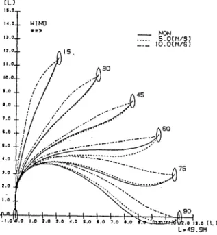
-t.oV/.O 1,0 2.0 3.0 4.0 S.O «.O 7.0 ».( _{>533aa3*M\X" .0 13.0 (U}

1=49.9H Fig.9 Paths of The Minimum-time Inward

Stopping with Wind Blowing on

6.2. Minimum Time Inward Stopping with Wind Blowing on

Figure 8 shows the maneuvering time until stop-ping at the given point in the minimum inward stopping with the wind blowing on. It is noticed that the time differences between the minimum stopping with wind velocity 5 m/sec and with wind of 10 m/sec are longer than those between the minimum stopping with no wind and that with windof5 m/sec. •E

In order to understand the reason for this, tke paths and other related maneuvering elements should be examined in detail.

I D e t ] R E L A T I V E W I N D D I R E C T I O N 2 0 0 . 0 1 0 0 . 0 0 . 0 : K O H A : 5 ｻ / i e c a - ' 0 " / ' " ・* 蝣蝣* * - N . - * N ' ¥ y ｻ ｰ ｰ "" " " 0.0 100.0 200. 0 [Sec)

Fig.10 The Relative Wind Directions

U - ｻ l 2 0 0 0 0 . 0 10 0 0 0 . 0 0 . 0 10 0 0 0 . 0 n :K O H - .A t S iA e c n : 1 0 ｫ/ s ｫ % . N ' " - - - . A ¥ 蝣- - -.-¥ / V . / - _ _ ・ 100.0 700. 0 (Sec! Fig.ll The Yaw Moments

IDc t) RUD DER ANC LE

(0.0 20.0 0.0 - 20. 0 - (0.0 ｫ. O i lOi/ iec u 0.0 100.0 200.0 [Set] Fig.12 The Time Histories of Rudder Angles

«n nxvsm

-looo. o

0.0

Fig.13 The Time Histories of Bow Tkruster Forces

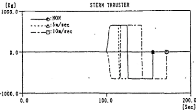
in) STERN THRUSTER

o.o- -1000.0-e:NON £: $»Aee o: 10«Aee

Li

Fig.14 The Time Histories of Stem Thruster Forces

Figure 9 shows the ship's paths. From this figure, it is found that the paths when the wind velocity is

10 m/sec, swell out in the outside directions. Fig-ures 10 and ll show the time histories of the wind directions relative to her head, and the yaw mo-ments when the initial bearing to the final point is 15 degrees. It is clearly recognized that when the wind velocity is 10 m/sec, the relative wind to her head changes to aftward from the abeam direction after 100 sec, due to her swelling out path. As the result, the yaw moment in the last stage, approaching the final point, changes from a star-board moment to aport one. It is clear that the minimum inward stopping maneuvers with a wind speed of 10 m/sec take account of this wind effect. Figures 12, 13 and 14 are the time histories of the rudder angles, and the bow and stem thruster forces, respectively. It is noticed that the ship is turned under full power at the last stage just before the terminal, utilizing starboard steering, and the starboard bow and port stern thrusting , in addition to the wind effect described above. 6.3. Minimum Time Inward Stopping with Wind Blowing off

As a final example, the minimum-time inward stopping problem with wind blowing off the final point is discussed.

Figure 15 shows the maneuvering time before stopping at the final point in minimum time. Also, Figure 16 shows the paths taken. It is noted that differing from the last problem, all the inward-stopping maneuvers with wind blowing off the fi-nal point almost coincide with the paths with no wind disturbances. The reason for these

coinci-dences is that a yawing moment to the port side is gained naturally, at the last approaching stage,

(126) K.Ohtsu

io£H

ISO.0

IS.0 å jo.'o

Initial approaching wigle

10/0 (OecJ

Fig.15 The Minimum Inward Stopping Times with the Wind Blowing Off

30 NON S.-OCH/S) IO.OCH/SJ IS

so

Fig.16 Paths of the Minimum-Time Inward Stopping with Wind Blowing Off

7. CONCLUSIONS

This paper has given the minimum-time ma-neuvering methods in two kinds of typical ship-handling problems under conditions with wind disturbances, for a small training ship with a rud-der, a controllable pitch propeller, and bow and stern thrusters.

In the itiinimum-tiine deviation problem, it was concluded to be sufficient for a ship's master to pay attention only to maintaining the ship's course along the minimum solution with no wind, irrespective of how the winds are blowing. In this problem, furthermore, actual sea trials were implemented. As an interesting result, it was found that despite the intermediate paths in the tests being slightly different from the optimal so-lutions, there are no large differences at the final point in each case. In the problem, of minimum-time inward stopping at a given position with the winds blowing on and blowing off, it was con-firmed that from the viewpoint of shiphandling practice, the optimal solutions are reasonable ma-neuvering methods that make maximumuse of

the effects of the wind, especially in the minimum inward stopping problems with the winds blowing

8. ACKNOWLEDGEMENTS

The authors wish to thank Dr.Mizoguchi,S. of the Ishikawajima Harixna Heavy Industries and C.E.of

the Shioji Maru, Mr.Hotta,T. and other crews of her for their helpful supports in the actual sea

tests.

9. REFERENCES

Shoji, K. and Ohtsu, K.(1992). Automatic Berthing Study by Optimal Control Theory. Proceedings of CAMS'92,Genova.

Ohtsu, K. and Shoji, K.(1994). Minimum Time Maneuvering of Ships. Proc. of MCMC'94. Fossen, T.I.(1994). Guidance and Control of

Ocean Vehicles. John Wiley and Sons. Wu, A.K.and Miele, A. (1980). Sequential

Con-jugate Gradient-Restoration Algorithm for Op-timal Control Problems with Non-Differential Constraints and General Boundary Conditions, Part 1, Optimal Control Applications and Method. Vol.1.

Miele, A. and Iyer, R.R.(197O). General Technique for Solving Nonlinear Two-Points Boundary-Value Problems via the Method of Particular Solutions. Journal of Optimization Theory and Applications, Vol.5, No.5.