ホップスの関数の正確な値について

全文

(1)Title. ホップスの関数の正確な値について. Author(s). 吉岡, 一男. Citation. 北海道教育大学紀要. 第二部. B, 生物学,地学,農学編, 36(1): 49-57. Issue Date. 1985-09. URL. http://s-ir.sap.hokkyodai.ac.jp/dspace/handle/123456789/6425. Rights. Hokkaido University of Education.

(2) Journal of Hokkaido University of Education (Section H B) Vol. 36, No. 1 BSW 60 tf- 9 fi. ^gSi.afit*^® (% 2 SUB) ^36^ ®1^ September, 1985. On The Accurate Values of Hopf's Function. Kazuo YOSHIOKA. Science Educational Laboratory, Asahikawa College Hokkaido University of Education, Asahikawa 070. ^R)—^ : '+-y 77®%ôjE5t^fitrî^ A?Si6af±ÂBJII^SS^-^ttS:5. Abstract We calculated the accurate values of Hopf's function q(r) by numerical integration. A micro-computer PC-9801 (NEC) with double precision floating numbers was used throughout the calculation. The numerical integration for the q(oo) value was decided both by Simpson's formula and by Gauss-Legendre's formula of order 6. For other q(r) values, we used Gauss -Legendre's formula of order 8.. The q(co) value obtained equals 0.710446089599. For 0<r^l0, q(r) values with nine significant figures were obtained. On the basis of the q(r) values obtained, the percentage errors of the q(r) values calculated by approximation formulae of 8 types have also been evaluated.. 1. Introduction. Hopf's function is the nonlinear part of the source function for the gray and plane-parallel atmosphere which is in radiative and in local thermodynamic equilibrium. It is defined by. S(r)=-|-F{r+q(r){,. (1). where r is the optical depth, F is the integrated flux and q(r) is Hopf's function ; S(T) is the source function which, in this case, is equal to the Planck function of the temperature at a layer.. Hopf's function plays an important role not only in the theory of the gray atmosphere but also in the evaluation of the accuracy of quadrature formulae for its mean intensity and the flux integrals. The mean intensity J(r) and the flux F(r) are expressed by the following integrals:. J(^)=-l f°S(r+t)Ei(t)dt+-i F S(r-t)Ei(t)dt, (2) '0. t.. Jo. (49).

(3) 50 Kazuo YOSHIOKA. F(r)=2 / S(r+t)E2(t)dt-2 / ~ S^-t^Wdt, (3) fo Jo where En (t) is the exponential integral function of order n, which is defined by. E,,a)=^°^dx.. (4). The condition of radiative equilibrium for the gray atmosphere leads to the following equations:. J(r)=S(r),. (5). F(r)=const(=F).. (6). When we express the integrals (2) and (3) in the form of operators A,.{S(t)j and <E^{S(t);, respectively, according to Kourganoff (1952), the equations (5) and (6) are written. A,{S(t);-S(r),. (7). 1>,{S(t);=F.. (8). According to these relations, differences between Ay{S(t)i and S(r) give errors of a quadrature formula for the mean intensity, while differences between <]>,.{ S(t)j and F give errors of a quadrature formula for the flux. On account of these characteristics, the source. function of the gray atmosphere in radiative equilibrium is often used for the evaluation of the accuracy of the quadrature formulae for J(r) and for F(r) (e. g. Nariai and Yoshioka. (1983)). Accurate values of Hopf's function q(r) are necessary for this evaluation. The q(0) value is derived theoretically to be I/y^3 (e. g. Chandrasekhar 1960), andtheq(co) value has been calculated to be 0.71044609 (Placzek and Seidel 1947). At present the most accurate values of q(r) for other optical depths are given to six decimal places. For example, Kourganoff (1952) has given a table of the q(-r) values obtained by the iterated variational method, and Mihalas (1978) has given one obtained by numerical integration. However, there are several differences in the q(r) values between these tables. More accurate values of q(r) are desirable for the evaluation of very accurate quadrature. formulae. In this paper, the q(r) values for 0 < r^lO and the q(oo) value have been obtained to nine and twelve decimal places, respectively, by numerical integration. The errors of the q(oo) values calculated by various approximation formulae have also been evaluated.. 2. Methods of Calculation and Results Different methods of numerical integration were used to find the q(o=>) value and the qCr) values for 0<r^l0. A micro-computer PC-9801 (NEC) with double precision floating numbers was used throughout the calculation.. 2.1. The q(oo) Value The q(oo) value was obtained from the following expression (Placzek and Seidel 1947) : •nf2,. ôo)=^-+ir2(^--rôt-.)d0- <9) (50).

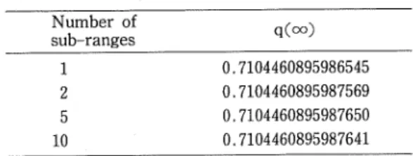
(4) 51. On The Accurate Values of Hopf's Function. Table 1 The degree of convergence of the q Table 2 The degree of convergence of the q (oo) value from the numerical integra(oo) value from the numerical integration by Gauss-Legendre's formula.. tion by Simpson's formula.. Number of. Number of. q(oo). sub-ranges*. 64 128 256. sub-ranges. 1 2 5 10. 0.7104460895994748 0.7104460895988048 0.7104460895987630. * It is equal to (n—l)/2, where n is the number of values. q(oo). 0.7104460895986545 0.7104460895987569 0.7104460895987650 0.7104460895987641. for the integrand used by Simpson's formula.. Fig.1 Graph of the integrand of equation (9),. QW.. The numerical integrations of this expression were decided both by Simpson's quadrature formula and by Gauss-Legendre's quadrature formula of order 6. In both cases, the entire. range of the integral was divided into sub-ranges with equal intervals to each of which the formula was applied. Since the integrand of equation (9), Q(0), is a fairly smooth function, as shown in figure 1, accurate values were obtained with comparatively small numbers of the sub-ranges in the case of Gauss-Legendre's formula. The degree of convergence for the. integration by Simpson's formula and by Gauss-Legendre's formula is indicated in table 1 and in table 2, respectively.. In the integration, the Q((9) values for 0^0.3 were calculated according to the expression (9). This expression, however, gives inaccurate Q(0) values for small 6 values, for we must carry out subtractions between very large numbers. For small 6 values (0<0.3), therefore,. the Q((9) values were calculated according to the following expression which is obtained by expanding 6 cot 6 in a power series in 0 :. QW=-. 3. 2+-. 1 , 202 , 0". 15 ' 315 ' 1575. T. 4ffL 138208 :+ 31185 ' 212837625 ' 608175' 206. (10). Errors in the Q(ff) values calculated in this way were estimated by comparison of the two Q (ff) values calculated from the above two expressions. They are smaller than 10~13. Judging. (51).

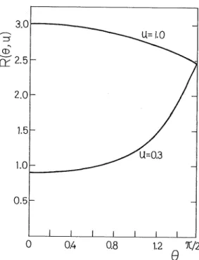
(5) Kazuo YOSHIOKA. .52. from this error and from the convergence indicated in table 1 and 2, it can be said that the following q(oo) value is correct to within one unit in the twelfth place of decimals : q(oo) ==0.710446089599. (11) 2.2. q(r) Values for 0<T^10 q(r) values for (Xr^slO were obtained from the following expression (Mark 1947) : q(r)=q(oo)--. 1. f:. 'du. >-T/U,. (12). 2/3" Jo H(u)Z(u)'. where H(u) is a limb-darkening function whose expression convenient for numerical calculation is. 11. f 1 /•'t'20 tan-l(u tan ff).. (13). H(u) =-7===exp -j -'- / " '"I" ^"_^"-id0 I-, ,/u+l""1' I TtJo l-Gcotff "" J ' /u+l. and Z(u) is given by. zw-('-iu'n(^))'+^w. (14). The evaluation of q(r) values by numerical integration of equation (12) needs another integral, i. e. that for H(u) (equation (13)). The integral for H(u) is also made by numerical integration. The entire range of the integral for H(u) was divided into two ranges, and each of these two ranges was further divided into sub-ranges with equal intervals to each. 3.0. ,U= 1.0. ~s 'S. CD. Q:. 2.5. 2.0. 1.5 "U=0,3. 1.0. 0.5. 0. Fig. 2 Graph of the integrand of equation (13),. I I 0.4. 11111 0.8. R(ff,u), for u=0.8. The R(0,u)for u=0.8 has a maximum at (9=1.25.. Except for u=0, R(i9, u) values are. Fig. 3. equal to 3u and to Tc1 '•/ '4 at 8=0 and at. 1.2. 9. 7C/2. Graph of the R(^,u) for u=0.3 and for u=l. For uÔ.68, R(<9, u) increases monotonically with 6, and for u<£ 0.89 it. 8=7c /2, respectively.. decreases monotonically.. (52).

(6) On The Accurate Values of Hopf's Function 53 of which Gauss-Legendre's quadrature formula of order 8 was applied. The numbers of the sub-ranges for the two ranges were taken to be equal. For 0.68 <u< 0.89, the boundary. between the two ranges was taken to be a maximum point of the integrand for H(u), R(5, u) (={0 tan-l(u tan ff)j/(l-0 cot ff)), where R(ff, u) has a maximum value, as is shown in figure 2. For the other values for u, where R(0, u) is a monotonic function, as is shown in figure 3,. the boundary was taken to be w/4 (for u^ 0.89) or to be a point where R(0,u) gives an average value of R(0, u) and R(7r/2, u) (for uÔ.68). The adequate number of sub-ranges for each of the two ranges was determined by the. following preliminary calculation. First, H(u) value was calculated, 2 being taken as this number. The H(u) value was then calculated again, this number being doubled. The process was repeated until a difference in H(u) values between two successive steps became smaller than 10-", after which the number for the last step was adopted. The adopted numbers thus determined are equal to or smaller than 4 for uÔ.3, but those for u<0.3 increased with decreasing u values. For example, the numbers were 8 and 256 for 0.2û<0.3 and for 0<u< 0.009, respectively.. In the integration of R(0,u), the R((9, u) values for O® (®=0.06 for uÔ.2 and ®= 0.06+0.06 X(u-0.2) for u>0.2) were calculated according to the expression (13). This expression, however, gives inaccurate R((?, u) values for small 9 values, for the accuracy of. the calculation of the denominator of this expression becomes too low. In this case (0<@), R(0, u) values were calculated according to the following expression which is obtained by expanding tan-l(u tan 0) and 8 cot 6 in a power series in u tan 6 and in 0, respectively :. R(0,u)=sp^),. (15). where S(<9, u) is given by. S(.,u)=u( l+f+^4+^6+^8)-f( ^+^4+t|^+^8 ) +^- (84+^0e+lfe8) -^ (e6+-ê8) +^8, d6) Table 3 Accurate values of the limb-darkening function H(u).. u. H(u). 0.0. 1. 0,1 1.24735044249 0.2 1.45035141281 0.3 1.64252226447 0.4 1.82927560320 0.5 2.01277877000 0.6 2.19413301932 0.7 2.37397491254 0.8 2.55270431684 0.9 2.73058766487 1.0 2.90781052908. (53).

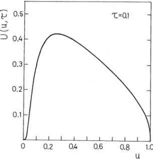
(7) 54. Kazuo YOSHIOKA. and T(0) is given by. TW=i+T502+W56. 1. :0S+-,. 2. (17). 4725" ' 93555'. Errors in the R(^, u) values calculated in this way were estimated by comparison of the two R(i9, u) values calculated from the above two expressions. They were smaller than 10-". As can be seen from the above process of the determination of the number of sub-ranges,. we are able to say that the H(u) values thus calculated are correct to within one unit in the eleventh place of decimals. These H(u) values are given in table 3.. In the numerical integration of equation (12), the entire range of the. ^. integral was divided into 4 ranges with unequal intervals, and each of the 4 ranges. was further divided into subranges with equal intervals to each of which Gauss -Legendre's quadrature formula of order 8 also was applied. As shown in figure 4,. the integrand of equation (12), U(u, r)(=. 0.2\-. exp(—r/u)/H(u)/Z(u)), decreases. 0.1 h. exponentially toward u=0 and decreases. logarithmically toward u=l. Judging from this behavior of U(u, r), the 4 ranges. 0. were adopted in many cases to be 0~0.03,. 0.2. 0.03-0.99, 0.99-0.999 and 0.999-1. Since. the U(u, r) values in the range of 0~0.03 are very small, this range is omitted for r> 0.6. The number of sub-ranges for. each of the 4 ranges was determined in the. Fig. 4. Graph of the integrand of equation (12), U(u, r), for r=0.1. It decreases exponentially toward u=0 and decreases logarithmically toward u=l.. same way as in the case of H(u). In this case the process was repeated until a. difference in q(r) value between two successive steps became smaller than 10-9,. so that it can be said that the q(r) values thus calculated are correct to within one. unit in the ninth place of decimals. The typical numbers of sub-ranges are 8, 32,. 256 and 256, respectively, for the ranges of 0-0.03, 0.03-0.99, 0.99-0.999 and 0.999. H(u) values which are independent of r were calculated once for all before the numerical integration for q(r) so that we would not have to repeat the numerical integration for H(u). (54).

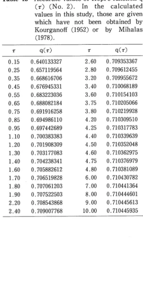
(8) 55. On The Accurate Values of Hopf's Function. Table 4a Accurate values of Hopf s function q (r) (No. 1). Asterisks attached to. Table 4b Accurate values of Hopf's function q. the values obtained by Kourganoff. values in this study, those are given which have not been obtained by. (r) (No. 2). In the calculated. (1952) or by Mihalas (1978). Kourganoff (1952) or by Mihalas (1978).. indicate that these values differ from those calculated in this study by more than IXlO-6. r. q(r). Q(-r). q(r). 0.15. 0.640133327. 2.60. 0.25. 0.657119564. 0.709612455. 0.577351. 0.35. 0.668616706. 2.80 3.20. 0.709955672. 0.588236. 0.45. 0.676945331. 3.40. 0.710068189. 0.55. 0.683223036. 3.60. 0.710154103. 0,65. 0.688082184. 3.75. 0.75. 0.691916258. 3.80. 0.710205066 0.710219928. 0.85. 0.694986110. 4.20. 0.710309510. 0.95. 0.697442689. 4.25. 0.710317783. 0.618468. 1.10. 0.700383383. 4.40. 1.20. 0.701908309. 0.710339639. 0.621854. 4.50. 0.710352048. 1.30. 0.703177083. 4.60. 0.710362975. this study. Kourganoff. Mihalas. 0.00. 0.577350270. 0.577351. 0.01. 0.588235475. 0.588236. 0.02. 0.595390802. 0.595391. 0.03. 0.601241385. 0.601242. 0.04. 0.606286279. 0.606287. 0.05. 0.610757413. 0.610758. 0.06. 0.614788767. 0.614789. 0.07. 0.618467295. 0.601242 0.610758. 0.709353367. 0.08. 0.621853757. 0.09. 0.624992852. 0.624993. 0.10. 0.627918738. 0.627919. 0.627919. 1.40. 0.704238341. 4.75. 0.710376979. 0.20. 0.649550411. 0.649550. 0.649550. 1.60. 0.705882612. 4.80. 0.710381089. 0.30. 0.663366042. 0.663365. 1.70. 0.706519828. 6.00. 0.710430782. 0.673091255. 0.663365. 0.40. 0.673090. 0.673090. 1.80. 0.707061203. 7.00. 0.680293581. 0,680293. 0.680240*. 1.90. 8.00. 0.710444601. 0.60. 0.685801. 0.685801. 2.20. 0.708543868. 9.00. 0.710445613. 0.70. 0.685801358 0.690108722. 0.707522503. 0.710441364. 0.50. 2.40. 0.709007768. 10.00. 0.710445935. 0.80. 0,693533945. 0.693535 0.696294. 1.25. 0.696293233 0.698539318 0.702571390. 0.702572. 1,50. 0.705130143. 0.705131. 0.90. 1.00. 0.690109. 0.698540. 1.75. 0.706801435. 2.00. 0.707916619. 0.707916. 2.25. 0.708673. 2.75. 0.708673120 0.709193115 0.709554426. 3.00. 0,709807751. 0.709806*. 2.50. 3,25. 0.709986731. 3.50. 0.710114019. 4.00 5.00 00. 0.710270519 0.710395177 0.710446090. 0.693534 0.698540 0.705130. 0.706802. 0.709191*. 0.707916 0.709191*. 0.709551* 0.709806*. 0.709985* 0.710120* 0.710270 0.710398* 0.710447. 0.710446. for each of r values. This shortened the time of calculation of one value for q(r) to thirty or forty minutes. Otherwise it would have taken several days with the micro-computer PC-9801.. The q(r) values thus obtained are given in table 4a and in table 4b together with those. obtained by Kourganoff (1952) and by Mihalas (1978).. (55).

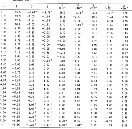
(9) 56 Kazuo YOSHIOKA Table 5 Percentage errors of the q(r) values calculated by various approximation formulae (e. g. at r=0, 15.5% and 29.3xl0-2% for the approximation number 1 and 4, respectively). The numbers representing the approximation formulae correspond to those given in the text. The numbers attached to figures indicate decimal exponent (e. g. 1.44xl0-6% at r=0 for the approximation of number 5).. 1. t. 2. 5. 4. 3. X10-2. X10-3. 6. xio-4. 7. X10-<. 8. X 10-'. 0. 15.5. -4.68-6. -8.71-'. 29.3. 95.5. 49.7. 0.98. 0,01. 13.3. -1.03. -1.09. 15.1. -2.81. -19.1. 7.73. 0.99. 0.02. 12.0. -1.44. -1.55. 9.22. -1.35. -33.0. 5.93. 0.99. 0,03. 10.9. -1.65. -1.81. 5.70. 7.04-5. -32.4. 7.14. 1.02. 0.04. 9.96. -1.76. -1.95. 3.37. 1.20. -27.4. 8.43. 1.04. 0.05. 9.15. -1.80. -2.03. 1.79. 2.03. -21.3. 9.25. 1.05. 0.06. 8.43. -1.79. -2.05. 0.68. 2.62. -15.3. 9.55. 1.04. 0.07. 7.79. -1.75. -2.04. -7.90--'. 2.99. -9.78. 9.41. 1.00. 0.08. 7.21. -1.69. -2.00. -0.60. 3.20. -4.97. 8.93. 0.94. 0.09. 6.67. -1.61. -1.95. -0.93. 3.29. -0.87. 8.20. 0.86. 0.10. 6,17. -1.51. -1.88. -1.13. 3.27. 2.53. 7.30. 0.77. 0.20. 2.64. -0.42. -0.91. -7.52-4. 0.82. 12.0. -2.71. -0.68. 0.30. 0.50. 0.46. -3.98-2. 1.98. -1.63. 5.53. -6.80. -1.38. 0.40. -0.95. 1.03. 0.57. 3.55. -2.89. -1.55. -6.46. -1.48. 0.50. -2.00. 1.34. 0.94. 4.54. -3.17. -5.89. -4.15. -1.05. 0.60. -2.79. 1.47. 1.14. 5.09. -2.84. -7.55. -1.44. -0.38. 0.70. -3.40. 1.49. 1.22. 5.33. -2.17. -7.31. 0.90. 0.31. 0.80. -3.87. 1.44. 1.22. 5.34. -1.36. -5.94. 2.62. 0.90. 0.90. -4.25. 1.34. 1.17. 5.20. -0.54. -4.00. 3.66. 1.33. 1.00. -4.56. 1.23. 1.09. 4.98. 0.24. -1.89. 4.12. 1.56. 1.50. -5.45. 0.68. 0.64. 3.41. 2.67. 5.37. 1.59. 0.60. 2.00. -5.83. 0.35. 0.33. 2.09. 3.06. 5.55. -2.02. -1.45. 2.50. -6.00. 0.17. 0.17. 1.22. 2.57. 2.32. -3.65. -2.68. 3.00. -6.08. 8.96-2. 8.28-2. 0.70. 1.89. -1.45. -3.66. -2.79. 3.50. -6.12. 4.67-2. 4.02-2. 0.40. 1.30. -4.63. -2,90. -1.89. 4.00. -6.14. 2.47-2. 1.82-2. 0.22. 0.86. -6.98. -1.94. 0.42. 4.50. -6.15. 1.32-2. 6.75-3. 0.12. 0.55. -8.58. -1,06. 5.88. 5.00. -6.16. 7.15-3. 6.78-<. 6.70-4. 0.35. -9.64. -0.35. 19.0. 00. -6.16. -1.26-5. -6.49-3. -5.48-5. 5.64 -". -3.22. 1.28. 1.28. 1.44-6. 3. The Accuracy of Various Approximation Formulae for Hopf's Function. On the basis of the q(r) values obtained in this study, the percentage errors of the q(r) values calculated by the following approximation formulae were evaluated. 1. Eddington approximation: q(r)=-^- (18) 2. Placzek (1947) : q(r) =0.710446-0.133096 exp(-3.68962r) (19) 3. Labs (1950) : q(r) =0.7104-0.1331 exp(-3.4488r) (20) 4. LeCaine (1947) : q(r)=0.7104457-0.243608E2(r)+0.224409E3(r) (21). (56).

(10) On The Accurate Values of Hopf's Function 57. 5. Norton (1963): q(r) =0.71044609-0.2830385 Ea(r)+0.57975839 EaCr). -0.75751038 E,W +0.45026781 Es(r) (22) 6. the fifth order variational solution by Kourganoff (1952) ; q(r) =0.710438-0.279901 Ez(r) +0.538809 EaCr) -0.646705 E4(r) +0.372129 EsCr). (23) 7. the sixth order variational solution by Kourganoff (1952) : q(r) =0.7104447-0.283903 Ez(r) +0.642454 EaC-r) -1.224316 E^Cr)+1.423034 Es(r) -0.590226 E<,(r) (24) 8. the sixth order lambda iterated variational solution by Kourganoff (1952) :. q(r) =0.5 EaCr) +0.710447{ 1-0.5 E^r) ; -0.283903 ^(r) +0.642454 ^(r) -1.224316 A4(r)+1.423034 ^(r)-0.590226 JleCr), (25) where A,,(T) is the A transform of E,,(r) : ^,(r)=A,{E,,(t){.. (26). The results are given in table 5. In this table, the numbers representing the approximation formulae correspond to those given above. Except for the approximation of number 8, the given errors are ascribed to the errors of the approximation formula itself. In the case of. the approximation of number 8, the errors for large r (say r>3) are due to the round off errors imposed by the computer. The absolute errors of the q(r) values calculated by these approximation formulae have been illustrated by Yoshioka and Nariai (1985).. Acknowledgement The author would like to thank Dr. K. Nariai of Tokyo Observatory, University of Tokyo, for suggesting this study and valuable discussions. The author also acknowledges the help of Professor T. Hasegawa of Asahikawa College, Hokkaido University of Education, in reading and criticizing the manuscript.. References. Chandrasekhar, S. (1960), Radiative transfer. p. 78 Dover Publications, Inc., New York. Kourganoff, V., (1952), Basic methods in transfer problems, p. 36 and p. 138 Oxford University Press, London. Mark, C., (1947), The neutron density near a plane surface. Phys. Rev., Vol. 72, p. 558—564. Mihalas, D., (1978), Stellar atmospheres, 2nd ed., p. 72 W. H. Freeman and Co., San Francisco. Nariai, K. and Yoshioka, K., (1983), Zur numerishen Berechnung der mittleren Intensitaten und StrahlungsstrOme in der planparallelen Sternatmospharen. Publ. Astron. Soc. Japan, Vol. 35, p. 113—130. Placzek, G. and Seidel, W., (1947), Milne's problem in trasport theory. Phys. Rev., Vol. 72, p. 550-555. Yoshioka, K. and Nariai, K., (1985), Accuracy of quadrature formulae for the intensity and the flux integrals. Ann. Tokyo Astron. Observatory 2nd Series, Vol. 20, p. 282-295.. (57).

(11)