Reitaku Institute of Political Economics and Social Studies
Working Report, No.30
Econometric Approach of Residential Rents Rigidity
-Micro Structure and Macro Consequences-
Chihiro Shimizu
25. January.2009
Reitaku Institute of Political Economics and Social Studies
Reitaku University,
Econometric Approach to Residential Rents Dynamics
*-Micro Structure and Macro Consequences-
Chihiro Shimizu†
-Abstract-
Why was the Japanese consumer price index for rents so stable even during the period of housing bubble in the 1980s? In addressing this question, we start from the analysis of microeconomic rigidity and then investigate its implications about aggregate price dynamics. We find that ninety percent of the units in our dataset had no change in rents per year, indicating that rent stickiness is three times as high as in the US. We also find that the probability of rent adjustment depends little on the deviation of the actual rent from its target level, suggesting that rent adjustments are not state dependent but time dependent. These two results indicate that both intensive and extensive margins of rent adjustments are very small, thus yielding a slow
response of the CPI to aggregate shocks. We show that the CPI inflation rate would have been higher by one percentage point during the bubble period and lower by more than one percentage point during the period of bubble bursting, if the Japanese housing rents were as flexible as in the US.
Keywords: hedonic price index, CPI (Consumer Price Index), price stickiness, time dependent pricing, state dependent pricing , Calvo model
JEL Classification Number: E30 ; R20
* I would like to thank Kiyohiko G. Nishimura(Bank of Japan), Tustomu Watanabe(Hitotsubashi University), Yoshitsugu Kanemoto, Yasushi Asami (University of Tokyo), and YongHeng Deng(University of Sothern California) for discussions and comments.
†Chihiro Shimizu, Associate Professor,The International School of Economics and Business Administration, Reitaku University, Hikarigaoka2-1-1, Kashiwa-city, Chiba, 277-8686 Japan.
Tel. +81-(0)4-7173-3439, Fax. +81-(0)4-7173-1100/E-mail: [email protected]
1.Objectives of the study
Recently, the link between economic indices such as consumer price index (CPI) and
economic and financial policies has been strengthening. Under these circumstances, attempts to clarify the mechanism of price changes are actively underway in Japan and overseas.3)
In particular, major industrial nations have commonly experienced a rapid increase and
subsequent decrease in asset values, particularly house prices, which has had a significant impact on the financial system and has led to economic recession. Therefore, intense discussions have focused on the development of indices that can formulate such price changes precisely (Diewert (2006)).
The standard Jorgensonian (frictionless) theory suggests that the user cost of an asset value is in agreement with the rental cost, and many attempts to analyze the relationship between the two have been made (for example, Verbrugge (2006)). In particular, house prices are obviously important independent economic indices in both the asset market and the goods and services market; house prices act as an important indicator that links the two markets (Goodhart (2001)).
In particular, since housing rent is an important constituent of the CPI (in Japan, it makes up approximately 26.3% of the CPI), the importance of housing rent is extremely high, not only as a benchmark in the housing market, but also as an economic index (Gordon and Goethem
(2005)).4)
Under these circumstances, some researchers have attempted to measure bias between the housing rent components of the CPI and the market housing rent. For example, Crone et al.
(2004) and Gordon and Goethem (2005) pointed out the importance of taking into account
3 http://www.ier.hit-u.ac.jp/~ifd/purposeplan_e.html
4 However, more consideration is needed on whether or not the rental cost observed in the rental market can serve as a surrogate indicator of the cost of servicing owned houses, as pointed out by Crone and Nakamura (2004).
changes in housing rent quality and estimated the bias of the CPI after estimating the hedonic quality-adjusted index. In the paper by Crone et al. (2006), the authors focused on changes in the method of estimating housing rent in the CPI, and analyzed the bias structure on the basis of the microdata used to estimate the housing rent in the CPI.
The housing rent observed in the CPI is calculated by simply adding the housing rent paid as a living cost, each component of which is based on a contract with different contract date.
Moreover, when considering the adjustment of rent, the summarized data include both housing rent agreed upon in a rollover contract that is completed when the tenant decides to remain in the same property after the initial two year contract has ended and the housing rent adopted in a new contract between a new tenant and a landlord. The housing rent for rollover is not altered during the period of the contract and the housing rent is rarely altered at the renewal of the contract as long as the same tenant continues to stay in the property because the adjustment of housing rent is markedly influenced by the institutional constraints imposed by the Land Lease and House Lease Law (Yamazaki (2000)). Consequently, it is estimated that the housing rent for a rollover
contract significantly deviates from the market housing rent.
Genesove (2003) analyzed the stickiness of housing rent for both types of contract, i.e., for new and rollover contracts, on the basis of individual data from an American housing survey and a follow-up questionnaire-based survey, and reported that an average of 29% of housing rents remained unchanged annually in the US. On the basis of these analyses, it was found that housing rent is sticky; although housing rent has an important weight in the CPI, many problems including methods of its estimation methods are involved in this analysis.
The purpose of this study is to analyze the mechanism of changes in housing rent by
formulating a demonstration model for the stickiness of housing rent in the house rental market.
We started by developing two databases on the housing market in the Tokyo metropolitan area (2.1) and estimating various housing rent and house price indices targeting the housing market in the 23 wards of Tokyo for the period of 1986 to 2006. We observed the long-term changes in the indices (2.2). A hedonic house price index and housing rent index were estimated, the changes in which were compared with the change in the housing rent components in the CPI. Our results revealed that house price and housing rent changed independently, and that the housing rent components in the CPI changed differently from the housing rent index obtained using the market housing rent.
Next, the mechanisms underlying the adjustment of the housing rent for rollover and new contracts were individually confirmed by observing them from the viewpoint of the house rental market (2.3).
On the basis of these fundamental analyses, the microstructure of the mechanism of housing rent adjustment was clarified. Specifically, the price stickiness of housing rent was measured (3.1). From the estimated statistics, it was found that housing rent in the Japanese market was extremely sticky.
We then clarified how this stickiness was generated. Whether or not the adjustment depends on market conditions (3.2) or on time regardless of the market conditions (3.3) was clarified by positive analysis. The results revealed that adjustments in housing rent occur randomly with time and are independent of market conditions, and thus follow a Poisson process. Therefore, a Calvo model was formulated to reestimate the degree of price stickiness (4).
Finally, we clarified the political consequences of our results. Specifically, we pointed out how the currently published CPI of Japan could be improved by modification on the basis of an equivalent approach, and the resultant implications on policy (5). In the conclusion, problems related to the study that require further clarification are also outlined (6).
2.1. Macrochanges in housing rent and house price and the stickiness of housing rent 2.1. Construction of database
The purpose of this study is to measure the stickiness of housing rent and clarify the microstructure behind its stickiness.
Before the start of the analysis, we collected data on housing rent for new contracts and the actual transaction price of houses in the 23 wards of Tokyo for 20 years from 1986 to 2006, including the “bubble” period. The main data source was the database of Recruit Co., Ltd., which publishes housing advertisement magazines.5)
Because the information is obtained from advertisements, it is considered that the data contained in the database are the asking prices of the properties. The data are updated weekly once they are registered in the database, which therefore includes historical price data for individual properties from the time the advertisement is first published until it is removed from the magazine or website because a new tenant6) has been found.
Among the various prices in the database, the final registered price, at which the property was removed from the magazine or website because a new tenant was found, was used for analysis in this study.7)
5 Recruit Co., Ltd. is the one of the largest vendors of housing information in Japan and has been publishing housing advertisement magazines for more than 40 years. It also runs advertisements for houses on its website..
6 There are two reasons for particular property information being removed from the magazine or website: a) a new tenant was found, or b) the owner decided to discontinue running the advertisement because he/she thought he/she would be unable to find a new tenant even if the advertisement was placed for a longer time. In the database of Recruit Co., Ltd., the reasons for the removal from the magazine or website are known. In this study, only the information removed from the magazine because of reason a) was used.
7 In the database of Recruit Co., Ltd, the actual contracted housing rent and the contracted house price of sample properties, in addition to historical price data, are included (approximately 24% and 28% of all the samples were for housing rent and house price, respectively). The comparison of contracted housing rent, contracted house price, final registered housing rent, and final registered house price indicates that the contracted price is in agreement with the final registered price in 99.9% and 97.8% of cases for housing rent and house price, respectively. In particular, in the case of housing rent, there is no room for negotiation, and the contract is concluded at the final registered housing rent. For this reason, the housing rent and house price used in this study represent the contracted housing rent and house price in the market.
To analyze the adjustment of housing rent and the structure of housing rent, which are the main themes of this study, the original housing rent data were extended so that the move-in date, date on which the tenant vacated the properly, and the change in the housing rent between the two days were observable. The housing rent data used in this study were restricted to the data registered in the database automatically when the former tenant expressed the intention to vacate the property and the property was ready for lease on the basis of the contract between Recruit Co., Ltd., and a major property management company. Therefore, the housing rent when the tenant of the property changed was obtained.
Here, we made a strong assumption. There are two types of adjustment of housing rent. One is the adjustment of the housing rent when a new contract is concluded between a landlord and a new tenant, and the other is the adjustment of the housing rent when a contract is renewed by a tenant who has decided to continue living in the same property after completing the period of the previous lease contract (rollover contract). In this analysis, we made the assumption that the housing rent is adjusted only when the tenant is replaced and that it does not change as long as the same tenant lives in the same property continuously. By making such an assumption, a panel database, which enables us to observe the residence period and the change in the housing rent for various properties, was constructed.
Although it is generally considered that housing rent is rarely adjusted at the time of a rollover contract, the reliability of our results when such a strong assumption is made may not be high.
Therefore, we constructed another database using adjustment behavior data for properties managed by major property management companies to determine the actual status of housing rent adjustment in the case of new and rollover contracts focusing on data for March 2008. The reason for focusing on contracts concluded in March is that the fiscal year in Japan is from April
to March, and the turnover of personnel and housing contracts is greatest in March. Therefore, a large bias may exist in the probability we obtained for contract renewal.
Data on housing rent adjustment for 15,639 properties in the Tokyo metropolitan area (Saitama, Chiba, Tokyo, and Kanagawa) were transcribed from contract documents to construct a database which includes the timing of new contracts, the housing rent before and after the conclusion of a new contract, the timing of contract renewals, and the housing rent before and after the time of contract renewal.8)
2.2. Macro changes in house price, housing rent, and CPI housing rent index
In this study, we started by examining the housing rent and macrochanges in the housing rent of properties in the 23 wards of Tokyo. Using the database of Recruit Co., Ltd., a hedonic housing rent index and house price index were estimated and compared with the CPI.
The data for properties in the 23 wards of Tokyo were collected for the period from 1986 to 2006 and consisted of the following: new lease contracts (housing rent), 718,811; transaction prices of non-timbered houses (non-timbered house price), 218,768; and transaction prices of timbered houses (timbered house price), 338,222.9)
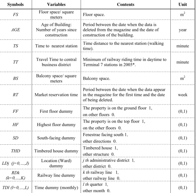
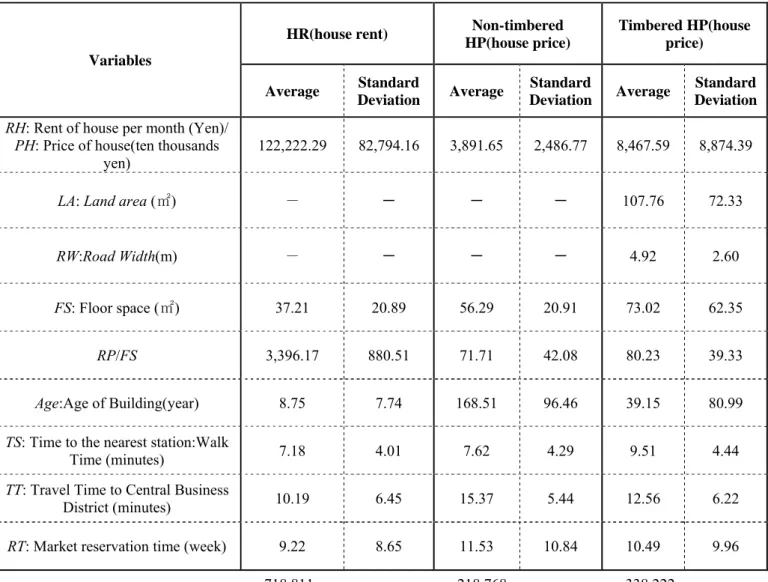
Other than the price information, information on attributes related to houses was summarized to estimate price indices in which the difference in quality of each housing unit is controlled (Table 1).The statistical values of the collected data are summarized in Table 2.
8 The database was provided by Daiwa Living Co., Ltd.
9 The data preparation in this study was supported by a Japan Society for the Promotion of Sciences Grant-in-Aid for Creative Scientific Research
“Understanding Inflation Dynamism in the Japanese Economy.” The coverage of data collected by Recruit Co., Ltd., exceeds 95% of the total transactions in the 23 wards of Tokyo according to Shimizu et al. (2004). On the basis of the result of the interview-based survey of Recruit Co., Ltd, the coverage of data for suburban properties collected by Recruit Co. Ltd. is extremely low, and the coverage of housing rent data is unknown.
In this study, to avoid the problem of sample selection bias and to maintain the compatibility of the data with CPI data, only the data for properties in the 23 wards of Tokyo were used for analysis.
The average monthly housing rent was 122,000 Yen with a large standard deviation of 82,000 Yen. The average price of non-timbered houses, mainly condominiums, was 38.9 million Yen, and the average price of timbered houses, mainly single-family houses, was 84.6 million Yen.
The average floor space of the properties was 37.21 m2 , indicating that they are mainly for single-person households, whereas the average floor space of non-timbered houses was 56 m2 and that of timbered houses was 73 m2; it is considered that such properties are mainly for
relatively large households. The average time to the nearest station for the three types of property was in the range of 7-9 minutes. Because data are collected for properties located in the 23 wards of Tokyo, properties with high transportation convenience are targeted in this study.
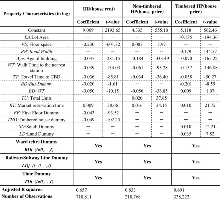
Next, a constraint-based hedonic price index was estimated on the basis of the following equation using the data collected between 1986 and 2006.10)
t
it Xi TD
P^ ^ ^ (1)
Here, Pit is the housing rent or house price for housing unit i in period t, Xi is an attribute vector of housing unit i, and TDt is a time dummy.
Table 3 summarizes the results of the estimation. The adjusted values of R2 for the housing rent function, the non-timbered house price function, and the timbered house price function are 0.657, 0.833, and 0.691, respectively. All three models can estimate the price with a relatively high power of explanation.
10 The repeat sales method or hedonic price method are representative methods of estimating the quality-adjusted house price (Diewert (2006)).
For the hedonic price method, there are several estimation methods, such as using a structure-constraint price index or a structure-nonconstraint price index. In this study, the most simplified structure-constraint price index was estimated. For details, please refer to Shimizu et al. (2007)
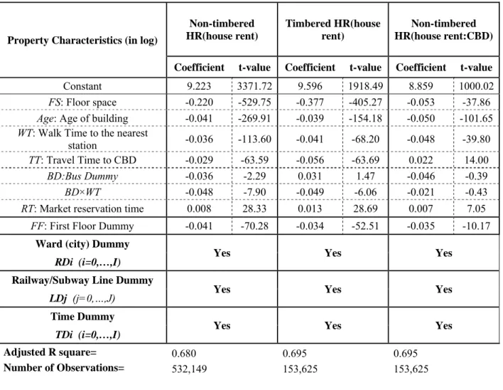
For the housing rent index, the non-timbered housing rent index and timbered housing rent index are estimated according to district, such as the central business district (CBD) including Chiyoda, Chuo, and Minato wards (Table 4), similar to the case of the house price index.
Changes in the hedonic rent index (HRI), non-timbered house price (NTHP) index, and timbered house price (THP) index over time are shown in Figure 1.
Both NTHP and THP indices rapidly increased from the first quarter of 1986 to the fourth quarter of 1987; assuming that the index in the first quarter of 1986 is 1, that in the fourth quarter of 1987 increased to 2.3 for the NTHP index and 2.5 for the THP index. After that, the indices decreased slightly then increased again, and in the fourth quarter of 1990, the NTHP index increased to 3.2 and the THP index increased to 2.6. In a series of studies conducted by Shimizu and Nishimura (2006)(2007), a constraint-based hedonic index was estimated using the actual transaction data of houses in a residential district using the same method as that adopted in this study, and similar results in terms of the rate of increase and the timing of the peak were obtained.11)
In contrast to the above indices, HRI increased from 1986 to 1992; assuming that the index in the first quarter of 1986 is 1, in the second quarter of 1992 HRI reached its maximum value of 1.39, after which it decreased. To find the relationship between HRI and prices of owned houses, average houses are considered and the hedonic housing rent/hedonic house price (rent/price ratio (%)) was calculated (Figure 2). The rent/price ratio exceeded 6% in 1986; after that, because of the increase in house prices, the rent/price ratio decreased to less than 3% in 1990. However, with subsequent decreasing house prices, the ratio increased again and surpassed 6.5% in 2001.
11 In papers by Shimizu and Nishimura (2006)(2007), the long-term land price index is estimated using the actual transaction price data for the land. The estimation indicates that the long-term land price index increased by a factor of 2.8 from 1986 to the fourth quarter of 1987; after that, the index decreased, then increased until the fourth quarter of 1990. The fact that the estimated results obtained using different data sources show the same tendency in terms of increasing rate and timing of the peak demonstrates the robustness of the result.
With the recent increase in house prices, the ratio again decreased to approximately 5.5% by the end of 2006.
Next, the HRI and CPI housing rent indices (CPI-Rent) are compared (Figure 3). HRI
increased by 40% from 1986 to the second quarter of 1992; however, CPI-Rent increased by only 15%. After that, HRI decreased but CPI-Rent continued to increase, although the trend in HRI has been roughly in agreement with that of CPI-Rent since the fourth quarter of 1994.
To observe the recent trends of these indices, an estimation is carried out using the THR and NTHR indices separately. The trend in the NTHR index focusing on central Tokyo (central business district (CBD)-NTHR, including Chiyoda, Chuo, and Minato Wards) was also analyzed to take into consideration variations between areas (the estimated results of HRI are summarized in Table4).
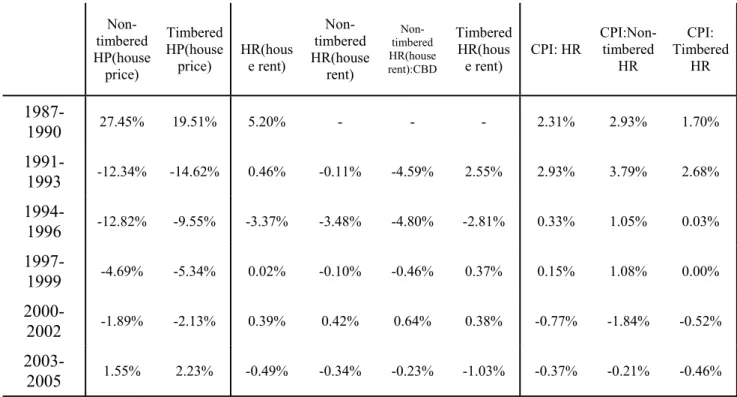
Figure 4 shows the NTHR, THR, CBD-NTHR, CPI-NTHR, and CPI-THR indices using their values in the first quarter of 2000 as a baseline. CBD-NTHR, NTHR, and THR for the 23 wards of Tokyo decreased by 40, 20, and 10%, respectively, from their peaks to their values in 2000.
However, both CPI-NTHR and CPI-THR continuously increased until 2000 while HRI decreased.
The trends in CPI-NTHR and CPI-THR are similar to that in HRI between 1994 and 2000.
However, after 2000, CPI-THR showed a significant decrease.
Table5 summarizes the average annual changes (%) in various indices for different periods. In 1987-1989 HRI increased by 5.2%, but the increases in CPI-NTHR and CPI-TH were far smaller, 1.7% and 2.93%, respectively. Furthermore, between 1991 and 1993, that for HRI was negative;
however, those of both CPI-NTHR and CPI-TH increased, indicating a continuous increase in these indices by 1996.
On the basis of this analysis, it was found that, although some correlation exists between the actual transaction price and the housing rent of a new contract, the strength of the relationship
between the actual transaction price and the CPI has been decreasing over time. As a result, decoupling between the asset price (in particular, the land price) and CPI may have occurred, and caution should be exercised when the CPI is used as an index to formulate policies.
2.3. Adjustment of housing rents for rollover contracts and new contracts
The comparison made shows that CPI-Rent behaves differently and independently of house price and housing rent indices. This is because CPI-Rent is determined on the basis of housing rents for both rollover and new contracts. For the 15,639 properties in the Tokyo metropolitan area (Saitama, Chiba, Tokyo, and Kanagawa) in March 2008, the status of the adjustment of housing rent due to new and rollover contracts was investigated to analyze the mechanism of housing rent adjustment for the two types of contract.
The housing rent level (Rit, Rit-1) before and after the adjustment of housing rent and the ratio of housing rent adjustment Rit / Rit-1 are summarized in Table6.
Among the 15,639 properties, new contracts comprise 526 properties (3.42%), and rollover contracts comprise 594 properties (3.86%). As explained previously, the turnover of personnel is greatest in March; therefore, a large sample selection bias may exist in the data. However, we consider that typical samples are extracted without bias regarding the range of adjustment of the housing rent.
Summarizing the statistics in Table 6, the average housing rent for the entire data set was about 90,000 Yen, whereas that for the new and rollover contracts was lower by approximately 6,000 Yen. In particular, for new contracts in which the old tenant was replaced by a new tenant, the average housing rent before the contract was approximately 83,000 Yen, whereas the average housing rent before the rollover contract was approximately 83,800 Yen, indicating that the housing rent for new contracts was somewhat lower. The average housing rent hardly changed
after the renewal of a rollover contract, whereas it increased by approximately 500 Yen after the conclusion of a new contract.
Table7 summarizes the ratio Rit / Rit-1 for new and rollover contracts.
In the case of rollover contracts, the housing rent remained unchanged in 96.97% of the
samples. This result agrees with our expectation at the start of this study. The reason behind this is that in Japan it is prohibited to increase housing rent without good reason, as stated by the Land Lease and House Lease Law, which strongly protects tenants. This result was also expected on the basis of a series of interview-based surveys.12) Genesove (2003) reported that the proportion of cases in which the housing rent remained unchanged at a rollover contract was 36% in the US.
Compared with the US, the stickiness of housing rent in Japan is extremely high.
In the case of new contracts, housing rent remained unchanged in 75.48% of samples, i.e. it was adjusted in approximately 25% of samples. The housing rent for new contracts can approximate the market housing rent, because no constraints are applied to the adjustment of housing rent. Under such circumstances, the figure of 75% seems high.13) However, the housing rent in new contracts remained unchanged in 14% of cases even in the US. Although the figure in Japan is high, the fact that housing rent is sometimes not adjusted when a new contract is concluded is not a phenomenon observed only in Japan (Genesove (2003)).
12 An interview-based survey was conducted in five representative real-estate management firms and real-estate companies in Japan, i.e., Daiwa Living Co., Ltd., Mitsui Fudosan Co., Ltd., Tokyu Land Corporation, Nomura Real Estate Development, and XYMAX Corporation. It was pointed out that the optimal strategy for the rental housing market in Japan is not to set a housing rent high to approximate the market housing rent, but to encourage a tenant to stay at the same property as long as possible. Due to constraints by the Land Lease and House Lease Law, housing rent cannot be increased without proper reasons, including an increase in fixed asset taxes, such as landholding taxes. Therefore, even when housing rents are increasing, housing rent tends to be sticky. Similarly, even when housing rents are decreasing, previously contracted housing rents are generally not changed when a roll-over contract is agreed upon.
13 According to an interview-based survey of managers of Daiwa Living Co., Ltd , the following reason for price stickiness was pointed out. In March 2008, which is during the analysis period, although housing rent remained almost unchanged, the property depreciated in value due to aging since the previous contract was agreed upon; thus, the housing rent in a new contract was often lower than the previous rent. As an optimum strategy for a real-estate management company, it is important to maintain the same housing rent. Once the housing rent for a new contract is adjusted downwards and other tenants in the same type of property know this fact, the real-estate management company inevitably accepts request from other tenants to decrease their housing rent. Therefore, concluding a new contract by maintaining the previous housing rent is particularly important. This explanation seems reasonable; however, more detailed analysis of this point will be required in the future.
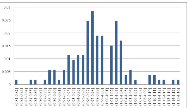
The change in housing rent before and after concluding a contract was observed in terms of Rit
/ Rit-1. Here, Rit is the housing rent for housing unit i in period t, and Rit-1 is the housing rent before the renewal of the contract for the same housing unit i. The distribution of Rit / Rit-1
(Figure 5,Figure 6) indicates that, in the case of a new contract, the housing rent is adjusted upward or downward; whereas in the case of a rollover contract, it is only observed to be revised downward. Furthermore, for new contracts, upward revision comprises 8.37% of cases and downward revision occurs in almost twice as many cases (16.16%). In the case of a new contract, the frequency of adjustments when Rit / Rit-1 is very close to 1 is small; rather, adjustment is carried out when the discrepancy between Rit and Rit-1 is large, which indicates that a menu cost exists in the market (Mankiw, 1985), and that the housing rent will not be adjusted unless it exceeds a predetermined price.
Next, the effect of market conditions on the adjustment of housing rent is analyzed, i.e., the relationship between the housing rent R* determined in the market and the housing rent R under the current contract is examined. If a discrepancy exists, i.e., R/R*≠1, and there is no stickiness in the market, the housing rent should be adjusted so that it reflects the market conditions.
It is not possible to directly observe R*. However, R* can be estimated. By modifying eq. (1), a hedonic housing rent function targeting the properties in the 23 Wards of Tokyo was formulated.14)
The relationship between the market housing rent, Rt-1*, and the housing rent before the contract, Rt , indicates that the average value of Rit / Rit-1 in the cases of new and rollover
14 The hedonic function expressed by eq. (1) was formulated using data from the 23 wards of Tokyo as a single function. However, a larger area, i.e., the entire Tokyo metropolitan area, should be targeted in the estimation. It has been demonstrated that when such a large market is targeted, the prediction accuracy will increase by dividing the market spatially into small sections (Goodman and Thibodeau (2003)). A railway line dummy was adopted as an important variable in the estimation using the Tokyo metropolitan area as a single unit. The area was divided into 55 models using the railway line dummy and a hedonic function was formulated. The data analyzed was for the period of April 2007 to March 2008.
For the time dummy, a monthly dummy was adopted instead of a quarterly dummy.
contracts is 1.04, indicating that the actual contracted housing rent is slightly higher than the market housing rent.
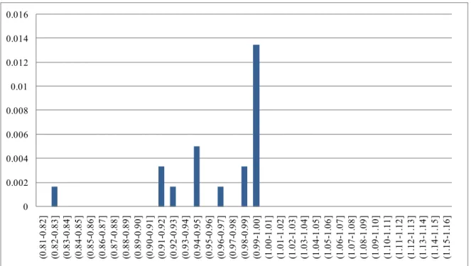
The distributions of Rt/Rt-1* and Rt/Rt-1 are shown in Figure 7 (new contracts) and Figure 8 (rollover contracts). Even when there was a discrepancy between the current housing rent and the market housing rent, housing rent was not adjusted in most cases. However, if one focuses on only the samples in which adjustments were made, the housing rent was revised so that the amount of discrepancy was adjusted.
Specifically, in both new and rollover contract samples, housing rents are sometimes adjusted when Rt/Rt-1 deviates substantially from 1; however, in most cases, the housing rent after new or rollover contracts remained unchanged even when Rt/Rt-1* deviated from 1. This tendency is particularly strong for rollover contracts.
On the basis of this analysis, we reconfirm that the probability of rent adjustment in the case of a rollover contract is extremely small, and that housing rent has strong stickiness during the lease contract period. In addition, there was no upward adjustment; only downward adjustment was observed. The influence of the Land Lease and House Lease Law, as predicted at the start of this study, was reflected significantly in the results.
When Rt/Rt-1* deviated upward from 1 in the case of a new contract, the housing rent is not adjusted to modify the discrepancy. The possibility of an estimation error associated with R* cannot be denied; however, we can conclude that this factor also plays a role in the strong stickiness of house prices. This problem of estimation error has not been resolved in this study and requires further examination in the future.
3.Degree of price stickiness of housing rent and its cause 3.1. Frequency of housing rent adjustment and price stickiness
It was found that housing rent, which is determined in the goods and services market, changes very slowly compared with price changes in the asset market. Furthermore, the change of HRI determined on the basis of housing rent in a new contract alone is different from that of CPI-Rent, determined on the basis of housing rent for both new and rollover contracts.
The period of lease contract in the Tokyo metropolitan area is basically two years, during which the probability of rent adjustment is low. In addition, adjustments to housing rents are markedly influenced by the institutional constraints imposed by laws such as the Land Lease and House Lease Law; the adjustment of housing rent, particularly increases in housing rent, rarely occurs even at the renewal of contract as long as the same tenant lives in the same property (Yamazaki (2000)). This was also demonstrated in the data provided by major property management companies. Consequently, it is expected that HRI determined on the basis of the housing rent of a new contract markedly deviates from the CPI-Rent.
Here, the degree of stickiness of housing rent is measured. The monthly change in Rt/Rt-1 was observed for data obtained from the database prepared by Recruit Co., Ltd. In the database, the timing at which the former tenant leaves and a new tenant arrives and the range of adjustment of the housing rent are included. However, it is not possible to observe the adjustment of housing rents at the time of agreement of rollover contracts. According to the analysis of data provided by major property management companies, the adjustment of housing rent can occur at the time of agreement of a rollover contract, although this only happened in approximately 3% of cases.
In this sense, in the analysis of data obtained from the database prepared by Recruit Co., Ltd, we should be aware that a constant level of error may be involved in the estimation of Rt/Rt-1, although the error level is thought to be minute.
Figure 9 shows the distribution of monthly rent changes calculated under the assumptions described (n=18,582,863).
The probability of a housing unit having no change in rent was 0.992, indicating high potential stickiness of the housing rent.
The distribution of monthly rent changes was concentrated around 1. This finding indicates that the number of large adjustments is limited, whereas the number of small adjustments is larger. The frequency very close to 1 is small; this was also observed in the analysis using a database from the major property management companies, indicating that a menu cost exists in the market.
The distribution of monthly changes in rent for different timings of contract is shown in Figure 10. As shown in the figure, the percentage of adjustment and its distribution vary depending on the timing of the contract. In particular, between 1989 and 1991, i.e., a period of rising housing rents, a large peak exists to the right of 1, and the distribution is skewed to the right. For other periods, the distributions are similar, and the frequency of adjustment toward a decrease in housing rent is large.
Figure 11 shows monthly price stickiness in terms of Rt/Rt-1 over time. Except during the bubble period, the stickiness of housing rent was almost constant and centered at approximately 0.992 from 1992 to 2006. This finding suggests that the stickiness of housing rent estimated in Figure 9 shows a similar tendency except during the bubble period.
When the probability of no rent change was converted to a yearly value, it was 0.9081 (0.99212).
Genesove (2003) studied the figure for the US and reported it to be 29%. The stickiness in the housing rent market in Japan is extremely high.
3.2. The State Dependent of housing rent- Estimation of adjustment hazard function-
The results of estimating probability of monthly rent change, housing rent is very stickiness.
For measuring stickiness in housing rents, we do to estimate an adjustment hazard, which was first proposed by Caballero and Engel (1993). The target rent for unit i in period t , which is denoted by Rit , is the level of rent that a landlord would choose if the landlord were allowed to adjust the rent as much as possible in period t . In other words, the target rent is the rental price we would see in an economy without any stickiness in housing rents. We define a zero-one index Iit as
otherwise 0
period in over turned is unit the if
1 i t
Iit
(2)
The adjustment hazard is defined to be the probability of a turnover ( Iit 1 ) conditional on the deviation of the actual rent from its target level
)
| 1 (
Pr Iit Rit1 Rit1 (3)
This conditional probability is useful when one wants to see a feature of state dependence in firms' pricing behavior.15) To estimate the conditional probability given in (2), we make the
15 For example, Saito and Watanabe (2008), shows an estimated adjustment hazard for goods sold at supermarkets such as milk, shampoo, and so on.The probability of price adjustment is very small when the price imbalance (i.e. the difference between the actual and target prices) is close to zero, but it monotonically increases with the imbalance, approaching to unity as the imbalance becomes very large. This means a state-dependent feature of firms' pricing behavior: namely, a firm seldom changes its price when it is close enough to the target level, but the firm is more likely to change the price when it faces a larger deviation.
following assumptions about Rit . First, we assume that Rit equals to Rit if a turnover occurs at unit i in period t (i.e., Iit 1 ). In this period, a landlord makes a new contract with a new tenant, and therefore is allowed to choose freely any level of the rent as far as it is acceptable to the new tenant. There is no reason for the landlord to pay attention to the level of the rent with the previous tenant. In this sense there is no stickiness in housing rents, so that the new rent Rit coincides with the target rent. Note that the new rent Rit can be regarded as “market'” rent in period t because it fully reflects the market condition in period t. In this sense “marking to market” occurs only when one tenant leaves and another one arrives.
The target rent Rit is not directly observable unless a turnover takes place at unit i in period t . However, it is still possible to estimate Rit as long as turnovers take place in other units, say the units j , k , and so on, and thus we are able to observe the target prices for those turnover units, Rjt , Rkt , and so on. Specifically, we first run a hedonic regression for period t using the rents for all of the turnover units, and then extrapolate it to obtain an estimate for the rent of the unit i in that period.
In sum, Rit is estimated as follows:
0 ˆ if
1 if
it it
it it
it R I
I
R R (4)
and Rit is estimated by expansion of equation (1). 16)
16 In estimating hedonic function using with equation (1), we set a strong hypothesis that the estimated hedonic parameters don’t change in the estimated term except for time dummies. This model is called “structural restricted model”. And in estimating equation (1), time dummies set as one-quarter. In estimating the target rent for making
“adjustment hazard”function, we have to estimate predict value (target rent) by hedonic function at higher accuracy level. Therefore, we calculate the target rent by “Over lapping Period Hedonic Model” (OPHM) proposed by Shimizu,et.al(2007) per month.
Given the estimate of Rit at hand, we are now ready to estimate an adjustment hazard function.
In estimating, we have a rent change problem of rollover contracts. In Recruit database, we can observe rent changes of only new contracts. The rollover contracts occur every two years after new contracts. So we cannot estimate the probability of the rent change for rollover contracts in over 2 years. In this case, if we calculate “adjustment hazard” function with all samples including rollover contracts, the estimated results have large estimated bias.
For treating this problem, we calculate the “adjustment hazard” function only less than 2 year’s samples after new contracts. For example, we calculate “adjustment hazard” function per months as Rt/Rt-1* and new contract’s events.The estimated result is shown in Figure 12.
We clearly see that the probability of adjustment, Pr(Iit) , does not depend on the deviation of the actual rent from its target (or market) level. This is in sharp contrast with the case of goods prices reported in Saito and Watanabe (2008). Non-state-dependent pricing, which is sometimes referred to as time-dependent pricing, is an important feature of housing rents.
3.3. The Time Dependent of Housing Rent- Estimation of hazard function-
The next thing we do is to conduct duration analysis. Specifically, they estimate hazard function, which is defined by
) 1 and
0
| 1 (
Pr Iit Iit1 Iitm Iitm1 (5)
Figure 13 shows the histogram of the completed price spells. We have 157,815 completed price spells. The length of these price spells ranges from 53 weeks (i.e., a tenant lives in a unit only for 53 weeks) to 1144 weeks (someone lives in a unit for more than 23 years!), and its median is 177 weeks.
Figure 15 shows the cumulative distribution function (CDF) for price duration. The vertical axis represents the cumulative probability in logarithm; for example, the value corresponding 400 weeks represents the fraction of price spells exceeding 400 weeks. The CDF seems to be on a straight line at least for the price spells whose length is less than 400 weeks. This indicates that price duration obeys an exponential distribution, implying that the rent adjustment is well approximated by a Poisson process.
Nelson-Aalen cumulative hazard estimates(Figure 15) conducts the same exercise as in smoothed hazard estimate(The Kaplan-Meier hazard estimates). The Kaplan-Meier hazard estimates indicates that the hazard function is almost flat at least for the duration less than 400 weeks, implying again that the rent adjustment is approximated by a Poisson process. These results could be interpreted as reflecting the fact that a turnover occurs due to purely random events such as marriage, childbirth, and job transfer.
From the estimated result, the probability of tenant changes is 0.0025 because, from 100 weeks to 400weeks, it is flat at that level. It indicates that the stickiness of rent change per week is 0.9975. This estimated result is the same as that is estimated in Figure9. And we calculate this estimated results per month is about 0.992, so we can understand that the probability of rent change is about 1%.
This estimated results is approximately the same level as of “adjustment hazard” estimate.
4.Estimating the Calvo parameter
The fact that the rent adjustment is approximated by a Poisson process suggests that one can apply the idea of Calvo pricing (Calvo 1983) to housing rents. As a first step, let me compare the rent estimated by hedonic rent and CPI rent in Figure 4. Figure 4 shows hedonic rent with the CPI rent. The estimated rent index rose significantly until the second quarter of 1992, and it started to decline after that, which is more or less consistent with fluctuations in selling prices. In contrast, the CPI rent did not exhibit such a large up and down during the bubble and the post-bubble periods.
Where does such a big difference come from? It is important to note that the hedonic rent index reflects changes only in the rents adopted in a new contract between a new tenant and a landlord, while the CPI rent contains the rents both for turnover and non-turnover units. Given the anecdotal evidence that the rent is seldom altered for non-turnover units, it would not be so surprising even if one finds slower adjustments (or more stickiness) in the CPI rent as compared with the hedonic rent.
To know whether this actually accounts for the difference between the hedonic and CPI rents, let us conduct a simple regression. We apply the Calvo model to housing rents by assuming that a turnover obeys a Poisson process with the probability α; namely, a tenant continues to stay at a unit with the probability of α and leaves a unit with the probability of 1-α. Furthermore we assume that a rent adjustment occurs with the probability of 1-θ even in a period in which an existing tenant continues to stay at a unit. Put differently, a rent adjustment occurs because of the two independent reasons: it takes place when one tenant leaves and a new one arrives; it also takes place at the timing of a renewal of a contract between an existing tenant and a landlord. The
anecdotal evidence indicates that the rent adjustment of the latter type seldom occurs; if so, the value of θ would be very close to unity.
Given these assumptions, the transition equation for the average rent of all housing units, including both turnover and non-turnover units, is given by
t t t
t R R R
R 1 (1 ) (1 ) (6) where Rt is the average of Rit over t , including turnover and non-turnover units, and Rt is the average of Rit over i for the turnover units in period t . Rt and Rt correspond to the CPI rent and the hedonic rent ( ˆ in equation (6)), respectively. Rearranging (7) gives us an estimating t equation
t t t
t R R
R 1(1) (7)
Note that we are only allowed to get an estimate for the product of α and θ but not for each of these two parameters. However, we have already learned something about the value of α in the previous subsection; the estimated hazard in Figure 15 implies that α=0.970 at the frequency of quarter.17) This means that the fraction of turnover units is 3 percent per week, much smaller than the numbers reported in the related studies.18) On the other hand, we get αθ=0.968 by estimating (7) for the period of 1986:1Q to 2006:4Q. These two estimates imply θ=0.997, indicating that a rent adjustment for non-turnover units occurs only with a very low probability.
17 The estimated hazard function in Slide 15 is almost flat at least for the durations less than 400 weeks, and it is about 0.0025. Then is equal to 0.9975 at the frequency of week, and (10.0025)120.970 at the frequency of quarter.
18 For example, Gali and Gertler (1999) reports that is about 0.8 for the whole industries in the United States: Gali, Gertler, and Lopez Salido (2001) finds that is in the rage of 0.5 to 0.9 for the European countries.
Figure 16 summarizes the regression results. The figure on the right hand side shows the values of the hedonic rent Rt , as well as the values of Rt which are calculated using the relationship
t
t
t R
R R
ˆ 1
1 ˆ ˆˆ 1
(8)
which is implied by equation (8). We see that fluctuations in Rt are considerably smoothed out, and that Rt is very close to the actual CPI rent.
Figure 17 on the left hand side shows an impulse response of R to a shock to R*. It takes 20 quarters to complete even half of its entire adjustment, which indicates very strong price stickiness.
5.Estimation of adjustment CPI by equivalent approach
It is appropriate to use R (instead of R*) when one is interested in calculating the cost of living for renter occupied housing. This is simply because what a renter pays in period t is based on the contract made in the past, and therefore the relevant rental price is not necessarily identical to the current market price Rt . However, as far as owner occupied housing is concerned, there is some reason to use the market price in evaluating its value. In particular, the so-called rental equivalence approach requires us to use the market price in evaluating the services provided by
owner occupied housing.19 The United States and Germany adopt this approach, while Japan adopts the so-called user costs approach. Specifically, the Japan's Statistics Bureau uses R even when evaluating the owner occupied housing services, based on the assumption that an owner pays the same amount as a renter does in period t. The fact that the deviation between R and R* was substantial during the bubble and the post-bubble periods suggests that the movement of CPI could be altered significantly by replacing R and R* in evaluating the owner occupied housing services.
Figure18 on the right hand side compares the price index using R* instead of R with the CPI.
One can see that the inflation rate in the new index is higher by about one percent in the latter half of the 1980s, and that it is lower by about two percent in 1993 to 1995. In particular, it fell to a negative value in the second quarter of 1993, while the CPI became negative only two years later. This reflects a noticeable difference between R and R* in that R* recorded a substantial decline in 1993 and 1994, while there was no such a decline in R. Deflation in 1993, rather than in 1995, could have urged the central bank and the government to make an earlier shift from monetary tightening to easing.
6. Concluding remarks
In this study, focusing on the stickiness of housing rent, which constitutes approximately 25%
of the CPI (an important economic indicator in economic policy, particularly in financial policy),
19 The rental equivalence approach values the services yielded by the use of a dwelling by the corresponding market rental value for the same sort of dwelling for the same period of time (if such a rental value exists)'' (Diewert and Nakamura (2008))
a positive analysis was carried out by constructing a panel database. On the basis of our results, we clarified the following.
First, a database of housing rents and house prices for the period of 1986 to 2006, including the bubble period, was constructed. HRI was estimated, and the comparison of HRI with other indices indicated the following;
-Both NTHP and THP rapidly increased from 1 in the first quarter of 1986 to 2.3 and 2.5, respectively, in the fourth quarter of 1987. After that, the indices decreased slightly then
increased again, and in the fourth quarter of 1990, the NTHP index increased to 3.2 and the THP index increased to 2.6.
-HRI increased from 1 in 1986 to a peak of 1.39 in the second quarter of 1992, after which it decreased. Next, HRI and CPI-Rent were compared. HRI increased by 40% from 1986 to the second quarter of 1992; however, CPI-Rent increased by only 15%. After that, HRI decreased but CPI-Rent continued to increase, although HRI has been roughly in agreement with CPI-Rent since the fourth quarter of 1994.
Next, to measure the stickiness of housing rent, a panel data set, which enabled us to observe the change in the housing rent for each property, was constructed. We found the following.
-On the basis of the observed monthly change in Rit/Rit-1, the percentage of cases without a rent change within a week was 0.992, indicating a high level of potential price stickiness of housing rent.
-The distribution of housing rent adjustment observed depending on the date of concluding a contract revealed that the ratio of adjustment and its distribution pattern depended on the timing of the contract; however, the monthly stickiness of housing rent has been almost constant, except during the bubble period, and Rit/Rit-1 had a value of approximately 0.992 between 1992 and 2006.
The adjustment hazard proposed by Caballero and Engel (1993) was estimated, and we found the following.
-The probability of rent adjustment Pr(Iit) does not depend on the size of the discrepancy between actual housing rent and the target (market) housing rent.
-It was estimated that the monthly probability of rent adjustment is approximately 0.9% per month, or 2.7% per quarter.
Because it was suggested that the adjustment of housing rent does not depend on market conditions, whether or not the adjustment varies depends on time was examined by formulating the hazard function.
-The probability of rent adjustment is random with respect to time; adjustments occur because of events such as marriage, childbirth, and relocation.
-This finding suggests that the adjustment of housing rent follows a Poisson process.
-The probability of replacement of a tenant per week is 0.25%, which is converted to approximately 1% per month.
These results indicate that a Calvo model can be applied in this analysis. Thus, the characteristics of CPI-Rent were examined by formulating a Calvo model.
-The probability of the adjustment of housing rent per quarter is 3.2%, including the adjustment of housing rent due to rollover contracts.
-The probability of rent adjustment in the case of a rollover contract is extremely low, about 0.03% per quarter.
Thus, the probability of the adjustment of housing rent per month was approximately 1%, on the basis of analysis using the adjustment hazard function, the hazard function, and the Calvo model.
This result indicates that the housing rent in Japan is sticky, and the figure is extremely small compared with the results reported for other related goods and services20). In particular, the stickiness of housing rent is increased by the existence of rollover contracts. This possibly induces bias in the CPI.
The housing rent used in the currently published CPI was replaced with the hedonic housing rent estimated in this study.
-Comparison of the modified CPI and the actual CPI indicates that the discrepancy between the two indices was large in late 1980s, during which the modified CPI markedly increased.
Between 1993 and 1995, the modified CPI decreased significantly, and was 2% lower than the actual CPI. Deflation occurred from 1993 to 1995; if the central bank or the government had known this, it may have been possible for them to ease monetary policy at an earlier stage.
Our results have various implications for macroeconomic policy. However, several problems still remain in this study.
We made the assumption that the housing rent for a new contract is adjusted so that it
approximates the market housing rent. However, the analysis of actual housing rent for a new contract revealed that the adjustment of housing rent does not always result in it more closely approximating the market housing rent. Furthermore, housing rent is not adjusted in
approximately 75% of new contracts. In other words, this finding indicates that the housing rent for new contracts is also sticky.
Although the reason behind this has not been clarified sufficiently, the following is considered to be a factor.
20 For example, Gali and Gertler (1999) reported that α for goods from almost all industries in the US is 0.8. Also, Gali, et al. (2001) reported that αin European countries is in the range of 0.5 to 0.9.
Grenadier (1995) pointed out that housing rent is determined on the basis of not only the current market conditions, but also of an option value based on the period of the lease contract and future expectations of the property value. Therefore, because the equilibrium housing rent is decided by the strategies of both the owner and the tenant, it is possible that housing rent is determined at a price that deviates from the market housing rent at the time of contract renewal. This possibility may explain why the housing rent deviates from the market housing rent at the time of the agreement of a new contract, but the reason for the lack of adjustment of housing rents cannot be easily explained.
As a possible reason, we considered that the housing rent at a new contract becomes sticky because the cost of searching for information on the housing market is extremely high, and therefore the cost of information correction is also high for the owner.
These problems have not been clarified sufficiently in this study. Because they are particularly important issues, we will address them in future studies.
References
[1].Abe, Naohito, and Akiyuki Tonogi (2008), “Micro and Macro Price Dynamics over Twenty Years in Japan- -A Large Scale Study Using Daily Scanner Data”, Research Center for Price Dynamics Working Paper No.
18, January 2008.
[2].Benigno, Pierpaolo (2004), Optimal Monetary Policy in a Currency Area, Journal of International Economics 63, 293-320.
[3].Caballero, Ricardo J., and Eduardo Engel (1993), “Microeconomic Rigidities and Aggregate Price Dynamics”, European Economic Review 37, 697-717.
[4].Calvo, Guillermo (1983), Staggered Prices in a Utility-Maximizing Framework, Journal of Monetary Economics 12, 383-398.
[5].Diewert, W. Erwin and Alice O. Nakamura (2008), “Accounting for Housing in a CPI”, Price and Productivity Measurement, Volume 1: Housing, Chapter 2, 13-48.
[6].Gali. Jordi, and Mark Gertler (1999), Inflation Dynamics: A Structural Econometric Analysis, Journal of Monetary Economics 44, 195-222.
[7].Gali, Jordi, Mark Gertler, and J. David Lopez-Salido, European Inflation Dynamics, European Economic Review 45, 1237-1270.
[8]. Goodman, A.C. and T.G.Thibodeau, (2003), “Housing market segmentation and hedonic prediction accuracy”, Journal of Housing Economics, Vol.12, pp.181-201.
[9].Ito, Takatoshi, and Keiko Nosse Hirono (1993), Efficiency of Tokyo Housing Market, Bank of Japan, Monetary and Economic Studies, Vol. 11, No. 1.
[10].Saito, Yukiko, and Tsutomu Watanabe (2008), Menu Costs and Price Change Distributions: Evidence from Japanese Scanner Data.
[11].Shimizu, C. and K.G.Nishimura, (2006), Biases in Appraisal Land Price Information: The Case of Japan, Journal of Property Investment and Finance, Vol.26, No.2, pp.150-175.
[12].Shimizu, C. and K.G.Nishimura, (2007), Pricing structure in Tokyo metropolitan land markets and its structural changes: pre-bubble, bubble, and post-bubble periods, Journal of Real EstateFinance and Economics, Vol.35 (4), pp.475-496.
[13]. Shimizu, C., K.G.Nishimura and Y.Asami, (2004), “Search and Vacancy Costs in the Tokyo Housing Market: An Attempt to Measure Social Costs of Imperfect Information”, Review of Urban &Regional Development Studies, Vol.16, No.3, pp.210-230.
[14].Shimizu, C.,K.G.Nishimura and T.Watanabe (2008),“Residential Rents and Price Rigidity: Micro Structure and Macro Consequences”, JSPS Grants-in-Aid for Creative Scientific Research Understanding Inflation Dynamics of the Japanese Economy, Working Paper Series , No.29.
[15].山崎福寿(2000)『土地と住宅市場の経済分析』東京大学出版会.
Table 1. List of analyzed data.
Symbols Variables Contents Unit
FS Floor space/ square
meters Floor space. m2
AGE
Age of Building:
Number of years since construction
Period between the date when the data is deleted from the magazine and the date of construction of the building.
year
TS Time to nearest station Time distance to the nearest station (walking
time). minute
TT Travel Time to central business district
Minimum of railway riding time in daytime to
Terminal 7 stations in 2005*. minute
BS Balcony space/ square
meters Balcony space. m2
RT Market reservation time
Period between the date when the data appear in the magazine for the first time and the date
of being deleted. week
FF First floor dummy The property is on the ground floor 1,
(0,1) on other floors 0.
HF Highest floor dummy The property is on the top floor 1,
(0,1) on the other floors 0.
SD South-facing dummy Fenestrae facing south 1,
(0,1) other directions 0.
THD Timbered house dummy Timbered house 1,
(0,1) other structure 0.
LDj (j=0,…,J) Location (Ward) dummy
j th administrative district 1,
(0,1) other district 0.
RDk
(k=0,…,K) Railway line dummy k th railway line 1,
(0,1) other railway line 0.
TDl (l=0,…,L) Time dummy (monthly) l th quarter 1,
(0,1) other month 0.
*Terminal Staion : Tokyo,Shinagawa,Shibuya,Shinjuku,Ikebukuro,Ueno, and Ootemachi Stations
Table 2. Summary of statistical values of house rent / price data: 1986-2006
Variables
HR(house rent) Non-timbered HP(house price)
Timbered HP(house price) Average Standard
Deviation Average Standard
Deviation Average Standard Deviation RH: Rent of house per month (Yen)/
PH: Price of house(ten thousands yen)
122,222.29 82,794.16 3,891.65 2,486.77 8,467.59 8,874.39
LA: Land area (㎡) - - - - 107.76 72.33
RW:Road Width(m) - - - - 4.92 2.60
FS: Floor space (㎡) 37.21 20.89 56.29 20.91 73.02 62.35
RP/FS 3,396.17 880.51 71.71 42.08 80.23 39.33
Age:Age of Building(year) 8.75 7.74 168.51 96.46 39.15 80.99 TS: Time to the nearest station:Walk
Time (minutes) 7.18 4.01 7.62 4.29 9.51 4.44
TT: Travel Time to Central Business
District (minutes) 10.19 6.45 15.37 5.44 12.56 6.22
RT: Market reservation time (week) 9.22 8.65 11.53 10.84 10.49 9.96
n=718,811 n=218,768 n=338,222


![Figure 8. R/R * vs. R t /R t-1 : Rollover contracts 0 0.00010.00020.00030.00040.00050.0006 (0.1,0.11] (0.2,0.21] (0.3,0.31] (0.4,0.41] (0.5,0.51] (0.6,0.61] (0.7,0.71] (0.8,0.81] (0.9,0.91] 1.00 (1.09,1.1] (1.19,1.2] (1.29,1.3] (1.39,1.4] (1.49,1.5] (1.](https://thumb-ap.123doks.com/thumbv2/123deta/6575755.2174933/41.892.214.694.161.548/figure-r-r-vs-r-r-rollover-contracts.webp)
