Bull. Kyushu Inst. Tech.
(M. & N. S.) No. 24, 1977, pp. 1-22
TWO-PLAYER ZEROSUM DISTRIBUTED PARAMETER
DIFFERENTIAL GAMES AND SENSITIVITY SYNTHESIS 0F OPTIMAL STRATEGIES
By
Toshihiro KoBAyAsHi*
Abstract
In this paper, we deal with two-player zerosum distributed parameter differential games and the sensitivity synthesis of optimal strategies for a game with terminal constraints.
The theory of static minimax problems in Hilbert spaces is applied to distributed parame- ter differential games with several types of controls. A two-player zerosum game with terminal constraints is considered from the playable point of view. The sensitivity synthe- sis is introduced to distributed parameter minimax differential games. In this synthesis, the sensitivity combined system plays an important role.
1. Introduction
As for distributed parameter differential games, there are works by Porter[1], Friedman [2] and Landy [3]. These works, however, were done for the systems with- out system parameter variations and uncertainty. It is necessary to consider another syn- thesis of optimal strategies with consideration of sensitivity to make up for the undesirable effects caused by system parameter variations and uncertainty. This is because sensitivity synthesis of optimal strategies are discussed in this paper,
In the first part of this paper, minimax problems are analyzed for functionals defined on real Hilbert spaces, where an existence theorem of saddle points is derived. As applica- tions of the above theory, distributed parameter differential games with distributed controls, boundary controls or pointwise controls are considered. In each case, the necessary and suMcient conditions for existence of saddle points are derived in the form of variational inequalities.
Secondly a game with terminal constraints is investigated, where the playability property plays an important role. The sensitivity synthesis of optimal strategies for the problem is developed to make up for the undesirable effects caused by the system parame- ter variations. In this sensitivity synthesis, the central role is played by the combined sys- tem which consists of a model equation and its parameter sensitivity equation. To ensure
* Dept. of Control Engineering
2 Toshihiro KoBAyAsHi
the existence of optimal strategies, the playability property of the combined system is ex- amined. By giving simple examples, the effectiveness of the present sensitivity synthesis is illustrated,
From another point of view, the differential game is regarded as the optjmal control problem with an uncertainty which is the opposite player to the control designer. By considering this we can make up for the undesirable effects caused by system parameter variations and uncertainty in some sense large.
2. MinimaxProblemsofFunctionals
In this section we consider minimax problems of functionals defined on real Hilbert spaces and extend the results for optimal control problems obtained by Lions [4]. The results stated here will be iiecessary later.
Let F, G be real Hilbert spaces and F.d, G.d be closed convex subsets respectively of F, G, Considerf, g--ÅrJ(f, g) be a functional from F.dÅ~ G.d into R such that the following conditions hold ;
(i) J,(f)= J(f, g) isaconvex functional infGF.d for eachgEG.d, (2,1) J2(g)=J(f, g) is a concave functional in gGG.d for eachfE I7.d. (2.2)
(ii) Ji(f)-'-År+co as Il.f'II År+co,fEF.d, (2,3) J2(g)----.-co as llgll----År+co,gGG.d. (2.4) (iii) f.J,(f) is strongly lower semi-continuous, (2.5)
g----År J2(g) is strongly upper semi-continuous,. (2• .6) We then have
[THEoREM 2,1] (Existence theorem ofa saddle point) There exists a pairf", g" such that
J(f*, g") =Inf. Sup.J(f, g)= Sup. Inf. J(f, g).
feFad gGGad geGad feFad
That is
J(f*, g)SJ(f", g") -Åq J(f, g") ,
If further Ji(f) is strictly convex and J2(g) is strictly concave, then the saddle point
is unique. In many problems the sets F.d, G.d will be bounded. In such cases the assump- tion (ii) wM be unnecessary.
Having obtained an existence result, it is necessary to characterize the saddle point.
we have
Two-Player Zerosuin DistributÅëd Parameter Diffcrential Games and Sensitivity Synthesis 3
[THEoREM 2.2]
Assume that the functional J,(f) is strictly convex and differentiable. Let the functional J2(g) be strictly concave and diflferentiable. Then the unique saddle point f"GF.d, g"
e G.d satisfying J(f*, g) E{g J(f", g") s; J(f; g") is characterized by
Jy(f*,g")•(f-f'`)})O forany feF.d, (2•7) Jg(f ", g")•(g -g") s{O for any ge G.d. (2.8)
In this chapter we shall be mainly interested in a special class of functionals:
J(f, g)-ip(fl f)- 'P(g, g)+2L(f, g)-2M(f) -- 2N(g) (2.9) where
a) 4År(fi, f2) is a continuous bilinear functional on F, which is symmetric, b) !U(gi, g2) is a continuous bilinear functional on G, which js symmetric, c) L(fl g) is a continuous bilincar functionai on I7 Å~ G,
d) M(f) is a continuous linear functional on I7, e) N(g) is a continuous linear functional on G,
f) (P(,fL f) ;}ir ci ll.f`ll2 for anyfE I', where ci is a positive constant, (2.10)
g) Yi(g, g) }ii c2Ug ll2 for anygE G, where c2 isapositive constant. (2.1 1) It is now easily verified that the functional J(f, g) defined by (2.9) satisfies the as-
sumptions of Theorem 2,1 and Theorem 2.2. From Theorem 2,1 it follows that there exists a unique sadcllc point (f", g"). In this case the derivatives Jl•(f, g), Jg(f, g) can
be explicitly calculated and we obtain [THEoREM 2.3]
The unique saddle point (f*, g") of the functional J(A g) defined by (2.9) js characterized by the following variational inequalities :
Åë(f",f--f")}lr-L(f-f",g")+M(f-f") forany fGF.d, (2.l2) !g(g",g-g*);}rL(f",g-g")-N(g-g") forany gGG.d, (2.13)
3. DistributedParameterDifferentialGames 3.1. Problemstatement
Let x =(xi,..., x.) denote the space variable; x ranges over an open set 9cEm with
boundary r: r is assumed to bc sufficjently regular. t denotes time; in gencral tG(O, T),
4 Toshihiro KoBAyAsHi
TÅq oo . We set 9 == st) Å~ (O, T), Z=Fx (O, T) . The controls will be denoted by f and g ' F.d and G.d represent the sets of admissible controls.
The state of the game corresponding to controls f and g is denoted by u(f, g)=u(t, x;f; g).
We are given Hilbert spaces Vand I respectively, V' is the dual space of V. We assume
1) Vcl, the injection Vinto I is continuous and Vis dense in I. I is identified with its dual space, and I may be identified with a subspace of V' and we have
VclcV'.
A family of bilinear forms on Vis given:
u,v Åra(t; u, v) foreach tG(O, T).
For this family we assume,
2) Vpt,vE V, the function t-Åra(t; ", v) is measurable on (O, T) and la(t; itt, v)l f{;l cll pt ll ' II vll
and there exists a Z such that
3) a(t; iu, Lt) +ZH Lt ll i2 År- ct II Jtt ll e, ct ÅrO, Jtt E V, tE (O, T).
For each t, we may write
4) a(t; pt, v)=(A(t)pt, v), A(t)ptGV',
where the bracket denotes the scalar product between Vand V', It may be seen that
5) A(t)Ey(L2(O, T; V); L2(O, T; V')), that is
if rEL2(O, T; V), A(t)r is the function t.A(t)r(t)eV'. Here Y(V, V') denotes a space of continuous linear mappings from Vinto V'.
We now introduce the space,
6) W(O, T)=={rlreL2(O, T; V), drldtGL2(O, T; V')}
Endowed with the norm
Ilrllw(o,T) =(S:Ilr(t)Iledt+S',"drldtili,dt)'f2,
W(O, T) is a Hilbert space.
Consider now the problem of evolution : find uE W(O, T) such that
duldt+A(t)"=f+g, f, g given in L2(O, T; V') (3.1)
Two-PIayer Zerosum Distributed Parameter Differential Games and Sensitivity Synthesis 5
and
u(O) =uo, uo given in l. (3,2)
For this problem, we have the following existence and uniqueness theorem.
[THEoREM 3.1] (Lions [4])
Under the hypothesis 2), 3), the above evolution problem admits a unique solution in W(O, T). Furthermore the solution is linear in f;g and uo, and depends continuously on f, g and uo•
3.2. Distributed parameter differential games We shall consider a differential game described by
duldt+A(t)u ---- Bif+ B2g (3.3)
u(f, g)1,..o=uo, u(f, g)GL2(O, T; V). (3.4)
Here Bi6Y(F; L2(O, T; V')), B2e.s2f'(6; L2(O, T; V')). By Theorem 3.1 u(f, g) can be sought in the form
u(f, g)=ui(f)+u2(g)+u3(uo) (3.5)
, vvhere ui, u2 and u3 are linear continuous operators.
Let the cost function of the game be;
J(f, g)-Ki llSu(f, g)-udll ft+(K2f, f)F -- (K3g, g)G (3•6)
, where Ki is a positive constant, ud is a given element in H which is a Hilbert space and S E Y( PV(O, T) ; H).
K2E-f2e(E F), (K2f, f)F l}r k211flli, k2ÅrO, (3.7) K3EY(G, G), (K3g, g)G ;}r k311gllZ•, k3ÅrO. (3.8)
We seek a saddle point (f", g") of J(f, g). Let us first rewrite J(f, g) in the form (2.9) by using (3,5), and then if we set
Åë( fi, f2) == Ki(SU i(f, ), SU ,(f, )).+ (K2 f,, f, ). (3.9) !I'(gi, g2) == -Ki(Su2(gi), Su2(g2))H+(K3gi, g2)G (3.10)
L(f, g)=Ki(Sui(f), Su2(g))H (3.11) M(f)=K,(Su,(f), u,-Su,(u,)). (3.12) N(g) :Ki(Su2(g), ud-Su3(uo))n (3.13)
we have
.
6 Toshihiro KoBAyAsHi
J(f, g) = Åë(f, f)- Y'(g, g)+2L(f, g)-2M(f)--2N(g)+KiIISu3(uo)-udlli-i• (3•14)
Since KiIISu3(uo)-udHft is clearly non-negative, we can apply Theorem 2.3 if the condi- tions (2.10) and (2.11) hold. (2.10) clearly holds for Åë(fi,f,) defined by (3.9). Define an operator TEY(G, H) by Tg=Su2(g) and then a suflicient condition for Y'(gi,g2)
in (3.10) satisfying the condition (2.11) is that
K3 -- KiT*ATis a positive definite operator. (3.15)
Here A is a canonical isomorphism ofH onto H' and ( )" is the adjoint operator ofan oper- ator ( ). Ifthe assumption (3.15) holds, the following theorems are obtained from Theo- rem 2.1 and Theorem 2.3.
[THEoREM 3.2]
Under the assumption (3.15), there is a unique pair of optimal strategy (f", g") of J(f, g).
[THEoREM 3.3]
Under the assumption (3.15), the optimal strategy (f", g*) satisfies the inequalities Ki(Su(f*, g*)-ud, Sui(f)-Sui(f"))H+(K2f", f-f")F 2) O
forany fGF.d, (3.16)
Ki(Su(f", g*)-ud, Su2(g)-Su2(g*))H-(K3g", g --g")G SgO forany geG.d. (3•17)
Next introduce the adjoint state by
-dp(f, g)ldt+A*(t)p(f, g)-K,S*A[Su(f, g)-u,] in (O, T) (3.18)
p(T;f; g)- O, p(f, g)EL2(O, T; V). (3.19)
Then Theorem 3.1 (with time reversed) asserts the existence and uniqueness of a solution p(f, g) in W(O, T).
Now put f =f*, g=g" in (3.18) and (3.19), multiply both sides of (3,18) by ui(f) -ui(f") and integrate over [O, T]. Using integration by parts and noting that
du,(f)ldt+A(t)u,(f)=:B,L u,(f)l,=, :O, (3,20)
we obtain
j"i,'(p(f*, g*), B,(f--f"))dt- (A7iBTp(f*, g"),f--f*)F (3•21)
AF being a canonical isomorphism of F onto F'.
Moreover noting that
Two-Player Zerosum Distributed Parameter Differential Games and Sensitivity Synthesis 7
K,S",'"(.S*ASu(f*, g*)-S"Attd, ui(f)-ui(f"))dt
= K,(Su(f*, g")-ud, Sui(f)-Sui(f"))H,
(3.16) may be written as
(Ai'Bfp(f",g*)+K,f*,f--f").;})O forany fe17.d. (3.22)
Similarly (3.17) may be written as
(AiiB:p(f",g")-K,g*,g-g")(if{;O forany gEG.d. (3.23)
Therefore we have proved
[THEoREM 3.4]
Under the assumption (3,15), (f", g") is a pair of optimal strategy if and only if
(Ai-iBfp(f",g")+K,f",f-f*),;}rO forany fEF.d,f*eF.d, (3.24)
(Aii B: p(f", Gsk• )- K3g*, g-g *' )G SO for any gE G.d, g* E G.d, (3•25) where p(f", g") is defined by
du(f*, g")ldt+A(t)u(f*, g")=Bif"+B2g* (3.26) u(O;f", g*) ==u,, u(f*, g")eL2(O, T; V) (3.27)
-dp(f", g")/dt+A"(t)p(f", g") =K,S"A[Su(f", g") -- ud] (3.28)
p(T;f", g")=:O, p(f", g*)eL2(O, T; V), (3,29)
If Fad =F, Gad :G
f"=:-Ki'A-FiBfp, g"=Ks'Ai'B:p.
3.3. Example of the game with distributed controls
Let V :H6(9), F= L2 (9), G =L2(9), B,, B2 == identity map. Here HT(9)= {u lu e Hm(9), Dku=O on LOsgks{m--l}, HM(9) being a Sobolev space of order m, Let A(t) be defined as follows:
A(t)u=-2:•'zi-i-oO-i-(aiJ•(t,x)-o-O.-"Jr) (3•30)
, where Iaij GLoo(S )) (space of functions defined on [O, T] which are essentially bounded) t 2 h• J'=i aij(t, x)4i4,• År- ct(e? + ••• + 4k), ct År O, 4i e R a. e. in 9.
A(t) is thus a second order elliptic differential operator.
8 Toshihiro KoBAyAsHi
The state of the game ig. given by
(7ulOt+A(t)u=f+g in e
(3.31) ulx --- O, u(O, x)= uo(x) xe 9.
If we take S== injection map of L2(O, T; V)-.L2(9), then H ==L2(9) :H' and A==identity map. The cost function is
J =Kij:S.(u(f, g)-ud)2dtdx+(K2f, f)L2(e)-(K3g, g)L2(Q) . (3,32)
Equations (3.28) and (3.29) reduce to
-OplOt+A"(t)p==Ki(u-ud) in 9 (3.33) pl, :O, p(T, x)=O xES2.
(3.24) and (3.25) reduce to
j:j.( P(f*, g")+K2f") (f-f ")dtdx }i O for any fE F.d, f" E F., (3. 34)
S:j.(P(f", g")-K3g*) (g -" g")dtdx KO for any g 6 G.d, g" e G.d. (3.35)
Moreover the condition (3.15) reduces to
j:j.(K3g-KiU"Ug)gdtdx;}ic2S','j.g2dtdx forany gEG, (3.36)
where U is the Green operator of A.
3.4. Example ofthe game with boundary conrtols
Let V=Hi(9), F==L2(Z), G :L2(Z), B,, B2 ==identity map. The state of the game is given by
aulOt+A(t)u=O in 9
(3,37) OulOvA=f+g on Z, u(O,x)=uo(x) xG2,
where
OulOvA=2Y,i--i ai,•(OulOxj)cos(v, xi) v being the normal at r exterior to 9.
Let S=:injection map of L2(O, T; V).L2(9), Then the cost functjon is J== Kij:S.(u(f, g) -- ud)2dtdx+(K2f, f)L2(E)-(K3g, g)L2ai) . (3.38)
The condition (3.15) reduces to
Two-Player Zerosum Distributed Parameter Differential Games and Sensitivity Synthesis 9
g:S.(K3g -- Ki U"Ug)GdZ 2}r c2g76S.g2dZ gE G. (3.3g. )
(3.24) and (3.25) reduce
j:j .(P +K2f") (f--f")dZ ;) O for any fE F.d, f" e F.d, (3.40)
S:S .(P -- K3g") (g -g")dZ :s{; O for any g E G.d, g" G G.d, (3,41)
where the adjoint state is now given by
, •--Op/0t+A*(t)p=Ki(u-ud) in 9
(3,42) Op/0v.,= O on X, p( T, x) ==O xe S2.
3.5. Example of the game with pointwise controls
Let V==L2(s;2), F==(L2(O, T))k and G=:(L2(O, T))h. The state of the game is given by
OulOt+A(t)u=: 2f• .. i fl(t) (ED 6(x ---- x`) + Z S•.igj(t) (Ei) 6(x - .v J') xi, yj E S2,
ulx=O, u(O, x) =u,(x) )cE9. (3.43)
The cost function is
J=KijT,'S,,(u(f, g)-ud)2dt dx +(K2f, f)F -- (K3g, g)G•
Then the condition (3,15) reduces to
(K3g -- Ki U" Ug, g)G År- c2 11gll3 gG G•
The adjoint state is now given by
-oplot+A*(t)p=Ki(u-ud) in e
pl,=O, p( T, x) =O xE 2. (3.44)
(3.24) and (3.25) reduces to
2lr•=,S:p(xi, t) (f,(t) -ff• (t))dt+(K,f*, f---f*). År-O (3.45)
ZO•==ij,P(Yj, t) (gj(t) ---gY•(t))dt -- (K3g", g --g")G f{gO (3.46)
4. Game with Terminal Constraints
In this section we shall consider the game with a terminal constraint u(T) =ud by a
10 Toshihiro KoBAyAsm
rule of the game. Therefore this game is described by
du(f; g)ldt+A(t)u(f, g)=:B,f+B,g te(O, T) (4.1)
u(O)=uo, u(T)=ud, (4,2)
J(f] g)-(K2f, f)F -- (K3g, g)G• (4,3)
This problem corresponds to the minimum energy control problem with terminal con- straints in the case of optimal control problems. Here we shall seek a minimax solution of this game. IfK3 is negative, it is natural to understand it as a cooperative game. On the other hand it may be considered as the optimal control problem wjth an unknown func- tion g, for which we consider the worst case. It is well known that there is a solution for the minimum energy control problem wjth a terminal constraint u(T)==ud, if the system is controllable at time T. In the following we investigate the existence condition for a mini- max solution of the game described by (4,1), (4.2) and (4.3).
Let F=F.d, G=G.d and Ei, E2 are separable Hilbert spaces. Let fGL2(O, T; Ei), geL2(O, T; E2), B,GY(Ei; I) and B2EY(E2; I).
Introduce the adjoint state by
-- dp!dt+A"(t)p == O, (4.4)
and let strategiesfand g be
f =• -KiiBf(t)p, g=Ks'BS(t)p. (4.5)
By using the Green operator U(t, T) of A(t) and an unknown element gt EI, a solution of (4,4) is described by
p(t)=U*'(T, t)g. (4.6)
Therefore
f(t) --KsiBT(t)U*(T, t)4, g(t) == KsiBg(t)U*( T, t)g•'•. (4.7) The solution of (4.1) and (4.2) is gjven by
u(t)= U(t, O)uo+j:U(t, T)(-BiKsiBf+B,KsiB:)U*(T, T)CdT. (4.8) Set tt(T)=ud and then
S:U(T, t)(-B,KiiBf+B,KsiB:)U*(T, t)4dt =u,--- U(T, O)u,. (4,9) Define an operator e on I by
eig' =S:U(T, t)(- BiKsiBf+B,KsiB!)u*(T, t)e'dt. (4.lo)
Two-Player Zerosum Distributed Parameter Differential Games and Sensitivity Synthesis 11
If the operator e js invertible, there exists a solution of our game. Further existence conditions are obtained by taking account of the following definition and theorem of controllability in the optimal control problems.
[DEFINITIoN 4.1]
A system
du/dt+A(t)u=B(t)f(t), u(O)==u,, (4,11)
(A(t)pt, pt) ;}ii ct 11 pt ll3 pa E V, tE (O, T), ct ÅrO (4. 12) is said to be controllable at time Tif
R(T) =- {u(T; f)lfG L2(O, T; F)}
is a dense subspace of I.
[THEoREM 4. 1]
The system (4,11) js controllable at time Tif and only if D( T) == SgU( T, t) B(t) B*(t) U*( T, t)dt År O.
From Definition 4.1 and Theorem 4,1, the following existence conditions are ob- tained.
[THEoREM 4.2]
There exists a solution of the game (4,1), (4.2) and (4.3) if the operator e has its inverse.
[THEoREM 4..3.]
When -BiKiiB\+B2Ks'Bg =-CC" for some C, there exists a solution of the game if a system (A, -BiKiiB\+B2KsiB:) is controllable at time T, where the system (4.11) is regarded as a system (A, -BB*).
In the case of Bi, B2, K2 and K3 being constants, we obtain a useful theorem;
[THEoREM 4.4]
There exists a solution of the game if i) BiKs iBi --- B2Ks iB2 #O and
ii) Either a system (A, -BiBi) or a system (A, -B2B2) is controllable at time T.
Next let us consider similar examples as the previous chapter.
(Example 4.1) (Distributed controls)
Consider a game described by
12 Toshihiro KLoBAyAsHi
Ou(f, g)10t+Au(f, g)=b,f+b,g in 9, f,gEL2(9),
u(.L g) ==O on X, u(O, x; f, g)=u,(x), u( T, x; f, g) == u,(x) in S2, J==k2ÅqTC f2(t, x)dtdx-k3Åq'Åq g2(t, x)dtdx.
JOJ9 JOJ9
Lions [4] showed that a system
Ou(f)10t+Au(f)=b,f in e, u(f)iE=O, u(O, x; f) =u,(x) in 9
is controllable at time T. From Theorem 4.4, it follows that there exists a solution of the game if b?IIÅq2 -- b31k3 #O•
(Example 4.2) (Boundary controls) Cong, ider a game
Ou(fL g)10t+Au(f, g)==O jn 9,
Ou(f, g)lavA=biJ'+b2g on Z, .LgEL2(2E]), u(O, x, ;f, g)==u,(.x), u(T, xif, g)=ud(x) in S2,
J==k2(Tg f2(t, x)dE-ic3ÅqTÅq g2(t, x)dz.
JoJr yoJr
Lions [4] showed that a system
Ou(f)/Ot+Au(f)=O in 9,
Ou(f)/av. = b,f on Z, u(O, x; f) =u,(x) in. 9
is controllable at time T. From Theorem 4.4, it follows that the game has a solution if
b?lk, -- b31k, eF O.
(Example 4,3) (Pointwise controls) Consider a game described by
Ou(f, g)10t+Au(f, g)=:b,f(t)(g)6(x-xi)+b2g(t)(g)6(x-x2), xi, x2ES2 u(f, g)IE=O, u(O, x;f, g)==u,(x) in 9
J := k2ÅqTf2(t)dt - k,C'g2(t)dt.
JO JO
Introduce the eigenvalues {Zj} and the eigenfunctions {ip,•(x)} of A which satisfy the
boundary condition, and then the system is reduced to infinite number of lumped systems:
Two-Player Zerosum Distributed Parameter Differential Games and S ensitivity Synthesis 13
duj(t)ldt + Zjuj(t) == bi dij(xi)f(t) + b2toJ•(x2)g(t)•
J' pm- ls 2•...
Ui(O) -umtu UO,`•
, where
u(t, x) = 2 ge., i ipj(x)uj(t), uo(x) = 2 ge• .. i to(X)Uo,•.
If ipj(xi)ipj(x2)#O and b?ip,2•(xi)lk2-b3ipi(x2)lk3#O (j--l, 2,...), there is a solution of each lumped parameter differential game forj=1, 2,... . Therefore there exists a solution of the distributed parameter differential game.
Generally speaking, if ip.(x ,)di .(x2) \ O and b? ip .2 (x i)lk2 - b3 ip .2 (x2)l k3 iF O for some n, the game for the n-th mode has a solution. If this holds for all n (n f{! N, N being a suit- able positive integer), the original distributed parameter game approximately holds.
5. Sensitivity Synthesis of Optimal Strategies
In the following part sensitivity synthesis of optimal strategies is considered to make up for the state variation corresponding to various system parameter variations. This sensitivity synthesis was studied for optimal control problems [5], Only feedforward strategies are here considered.
5.1. Sensitivity functions and sensitivity equations (A) ct•-sensitivity function and ct-sensitivity equation
We shall deal with the sensitivity for ordinary parameter variation without variation of initial conditions and the order of the system.
Consider a system presented by
duldt+A(t; ct)=B,(ct)f+ B2(ct)g, u(O) =uo (5.1)
, where ct is a variable parameter, cteH.; H. being a Hilbert space. We shall regard the system (5.1) with parameter value ct as the model system for a physical one. On the other hand we describe the actual system by (5.1) with parameter value ct+Act, ActeH.. The difference in the state between the actual system and the model system corresponding to certain controls is described by
Au(t; ct) ==u(t; ct ---Act)-u(t; ct) = v( t)A ct + O[ll A ct ll i2i.]
where v(t)= u.(t; ct) is the ct-sensitivity function. If A, Bi and B2 are differentiable in the parameter ct, the sensitivity function satisfies
dvldt+A(t; ct)v+A.(t; ct)u =:Bi.(ct)f+ B2.(ct)g (5.2)
v(o) =o,
14 Toshihiro KoBAyAsHi
Equation (5.2) is the ct-sensitivity equation.
(B) 6-sensitivity function and 6-sensitivity equation
Consider the case there is a difference At{o only with respect to the initial condition
x
between the model system and the actual one. Here Auo=6h, hel and Åí is a scalar in some sense small, That is, the model system is described by
du/dt+A(t)u =Bif+ B2g, u(O)=Uo•
The actual system is denoted by
du!dt+A(t)u == B,f+ B,g, u(O)=uo+Auo. (5,3)
Then the difference in the state between both systems is denoted by Au(t; tto) :,/v(t)Auo+O[llAuo1l7]
, where w(t)=u.,(t; uo) is the 6-sensitivity function. The fi-sensitivity equation
dwlclt+ A(t)w=O, w(O) =h (5.4)
is obtained.
(C) 6-sensitivity function and 6-sensitivity equation
Suppose that the actual system is described by a differentialdi-difference equation:
duldt+A(t)u+u(t-e) == Bif+ B2g (5.5) u(t)=h(t) tE(----qO), u(O)=u, (5.6)
, where 6 is a scalar time delay parameter which is positive and in some sense small. Con- sider the model system
duldt+ A(t)u +u == B,f+ B,g, u(O) =:uo (5.7)
which is obtained by letting e= O in (5.5) and (5.6). Then the difference in the state be- tween both systems is denoted by
Au(t; 6) = sz(t) + O(62) ,
where z(t) ==u,(t; O) is the 6-sensitivity function. The S-sensitivity equation
dzldt+A(t)z+z+A(t)u+u == Bif+ B2g, z(O)= O (5.8)
is obtained, which is not a differential-difference equation.
5.2. Combinedsystems
Consider the model equation and the sensitivity equation simultaneously, which is
simply called the combined system, then it may be recognized that there is a possibility to
control not only the model state but also its sensitivity function by choosing proper con--
trols. That is, we can take the effect ofthe small system parameter variations in the model
Two-Player Zerosum Distributed Parameter Differential Games and Sensitivity Synthesis 15
equations into consideration at the initial stage of the synthesis. This is the basis of the sensitivity synthesis of optimal control. We extend this sensitivity synthesis to the differ- ential games with terminal constraints. In cooperative games, the meaning ofthis synthe- sis can be easily understood. As, in our minimax game, the terminal state is previously given by a rule of the game, we can consider that both players want to make the state sen- sitivity small cooperatively. This is because they do not want to change the system state which has been synthesized once.
Combining the model equation and the ct-sensitivity equation, we can get the ct-com- bined system:
duldt+A(t)u =Bi f+ B2g, u(O) =uo {
(5.9) dvldt+A(t)V+A.(t)U=Bictf+ B2ag, V(O) "O
which governs the extended state (u, v),
Similarly we can get the 6-combined system and the S-combined one. We show that we can apply the results of Chapter 4 to the combined systems. We consider, for example, the ct-combined system. Let x=(ij), w=(1. AO), Y =(SII3t+BB2,g.,e) and then (5i9) reduces to
dXldt+ WX == Y, X(O) == (o"O). (5.10)
If X(O) :O, then
C'(dxldt, x)dt == Åq'{(duldt, u)+(dvldt, v)}dt=$(lu(T)12 + lv(T)12) ;;2: O•
JO JO
Moreover if AE .s2f'(V, V'), A.G Y(V, V'), (Au, u) l}i 6iHuII3 and ((A +A.)u, u) }ir fi2 11uH& 6i, 62 ÅrO for any ue V, C'( wx, x)dt = Åq'{((A + A.)u, u) + (A v, v)}dt
JO JO
;}i: 6,Åq'11u [I 3dt+ jBiCTIIvli 3dt ;;ir O. (s.11)
JO JO
Hence the existence and uniqueness of a solution of (5.10) follows [4]. This is also true for the 6- and the 6-combined systems. From this we can apply the results of Chapter 4 to the combined systems.
5.3. Sensitivitygames
We have stated that we can make the sensitivity synthesis of optimal strategies by con-
sidering the combined systems. How to take the sensitivity into consideration depends on
the original problems. For example, a saddle point can be sought for a new performance
16 Toshihiro KoBAyAsm
index
J,(f, g) =J(f; g)+K4j:v2(t)dt. (5,I2)
Here we consider the sensitivity synthesis of optimal strategies for the game with terminal constraints. Sensitivity games may be thought that each player add a sensitivity constraint v(T) =O to compensate the violence of the terminal constraint (u(T) == O required by a rule of the game) in spite of the parameter variations. On the other hand, consider the optimal control problem for the system equation with an unknown function g(t) and unknown system parameters. Then the minimax game is considered for the unknown function g which is supposed to be the opposite player to the control designer. Furthermore the sensitivity synthesis is considered to make up for the undesirable effects caused by small system parameter variations.
For the game:
duldt+A(t)u == B,f+B2g te (O, T) (5.13)
u(O) == uo, u(T)=ud, (5. 14)
J(f, g)=(K2f, f)in-(K3g, g)G. (5.15)
the sensitivity game is stated as follows:
duldt+A(t)u=B,f+B,g te(O, T) (5.16)
u(O)=uo, u(T)=ud, (5.17)
dvldt+A(t)v+A.(t)u=B,.f+B2.g te(O, T) (5.18)
v(O) == O, v( T) =O, (5.19)
J,(f, g) == (K2f, f)F-(K3g, g)G• (5.20)
The 6- and the 6-sensitivity games can be simjlarly stated. We can apply Theorem 4.2, 4.3, 4.4 to investigate the existence of solutions for the sensitivity games. We shall con- cretely study this in each case.
Let us consider a following actual system :
Ou(t, x)10t+aAu(t, x) :b,f(t, x)+b2g(t, x) in 9 (5.21)
u(O, x)=O, )cESI2, Ou(t, x)10vA+13(t, x)u(t, x)=O on X where A is given by (3.30), 6(t, x) }i O on Z and f, g E L2(e).
A cost function is given by
J== j:j.[kif2(t, x) --- k2g2(t, x)]dt dx. (s.22)
Two-Player Zerosum Distributed Parameter Differential Games and Sensitiyity Synthesis 17
(Case I) a being a variable parameter
The sensitivity equation for the variable parameter a becomes Gv(t, x)/O't+a,4v(t, x)+Au(t, x) =O in 9
(5.23)
v(O, .y) == O, xE SI2, 0v(t, x)/OvA + 6(t, x) v(t, x) = O on Z
From Theorem 4,4 it follows that this sensitivity game has a solution if bilki -- bi/k2 ,F O and the system
Ou/Ot+aAu=bif in 2
OvlOt+aAv+Au==O in e (5.24)
u(O, x) =O, v(O, .x) :O xESI}
Ou/c? vA + 13u=O, OvlOvA + IIv= O on Z
is controllable at time T. From the definition 4.1, the system (5.24) is controllable at time Tas u(T, x;f) and v(T, x;f) generate respectively dense subspaces of L2(9). To see this, define ip, W such that
.g
u(T, x;f)ef)(x)dx==O (beL2(9) forany f (5,25)
S2
s
v(7;x;f)V(x)dx=O uteL2(S2) forany f. (5.26)
se
We introduce p and q as the solutions of
-0plOt+aA"p+A"q=:O in 9, p(T,x)=ip(x) (5,27)
OplOvA.+t3p=O on 2S (5.28)
--- OqlOt+aA "q =O in 9, q( T, x)= W(x) (5,29)
OqlOv.,+Xlq==O on Z. (5.30)
Then
O= jQ( - OplOt + aA"p + A"q)u(f)dt dx + SQ( -- OqlOt+ aA"q)v(f)dt dx
" Sep(eulOt+ aAu)dt dx + jeq(OvlOt + aAv+ Au)dt dx
S9
-S.ip(X)U(T, X;f)dx- W(x)v(T, x;f)dx
==btSQpfdtd•x forany .1';
18 Toshjhiro KoBAyAsHi
hence p==O. From this and (5.27), A"q=O. If AidiFO(i---1, 2,..,); 2i being eigenvalues of A, then q=O. Therefore ip =O and V=O. We now get the required result from the Hahn-Banach Theorem.
(Case II) bi being a yariable parameter
Let a==1. The sensitivity equation for a variable parameter bi becomes ov(t, x)/et+,4v(t, x)==f(t, x) in e, v(o, x)==o xGsll
(5.31) Ov(t, x)lavA+13(t, x)v(t, x)==O on ,x.
We shall show that the existence of the solution of the sensitivity game follows and more- over the sensitivity function v(t, x)=:O in e.
Introduce the adjoint system:
-eplOt+A*p=O in 9, aplOv.,+/7p==O on Z (5.32)
-0qlOt+A"q=O in 9, Og/OvA.+ISq=O oii E.
and suppose that strategiesfand g are given by
f== -- (bip+q)lki, g=b2p!IÅq2. (s.33)
The solution of (5.32) is described by
P=U"(T, t)pT, q:=U*(T, t)qT p7-, qTEL2(S;2). (5.34)
By using (5.33) and (5.34), u(T) and v(T) are given by
u( T) = S: U( T, t) U*( T, t)dt{( - b?lki + b3/k2)p T -- biq Tlki} (5• 35)
v(T)=S:U(T, t)U*(T, t)dt(-bipTlki-qTllci), (5.36)
Since
S:U(T, t)U*(T, t)dtÅrO, (5.37) --(bipT+qT)lki=O in S;2 (s.3s)
which makes v( T) == O. From this it follows that f= O, v == O in e. Then
u(T) =S:U(T, t)U*(T, t)dt•bZp.lk2. (5.39)
Hence the existence of tlie solution of the sensitivity game follows if b2 eF O, and the sen-
sitivity function v(t, x) and the control f(t, x) vanish in 9. This result holds for the game
in which b2 is a variable parameter. Then if bi )F O, the sensitivity function v(t, x) and the
Two-Player Zerosum Distributed Parameter Differential Games and Sensitivity Synthesis 19
control g(t, x) vanish in e.
(Case III) uo(x) being a variable initial function
Let u(O, x)=:uo(x) in (5.24), The 6-sensitivity equation becomes Ow(t, x)IGt+Aw(t, x) =O .in 9, w(O, x)==h(x) hEL2(!l2) eW(t, X)/0VA+6(t, X)M7(t, X)=O Oii Z.
From this form, it is clear that the combined system is not controllable. Hence the sen- sitivity game does not have a solution.
(Case IV) E being a small time-delay parameter Consider an actual system described by
au(t, x)10t+Au(t, x)+u(t-s, x)= b,f(t, x)+b,f(t, .y) in 9 (5.40)
u(t, x)=h(t, x) tG(-6, O), u(O, x) =O xEst? (5.41) 0u(t, x)!0vA+19(t, x')u(t, x)==O on X. (5.42)
The j-sensitiyity equation becomes
O..(t, x)/0t + A :• (t, x) + :• (4 .)c)+Au(t, :)c) + u(t, x) = h, f( t, x) + h2g(t, )c) (5 .43)
z(O, .x)=7-O .xGS2, Oz•(t, x)/OvA+LS(t, x'). :•(t, x)=O on E. (.S. .44) From a similar consideration as Case I, it fbllows that the sensitivity game has a so!ution
if
b?lki -- b3!k2 SE O and Zi \-1 (i•= 1, 2,,..); Ai bejng eigenvalues of A.
5.4. Numericalresults
In this chapter we shall shovv that the sensitivity synthesis is f,uperior to the coiiven- tional one by giving several numerical examples.
(Example 5.1) ct-variation
We consider the following game with a terminal constraint u(1, x) == sin nx:
0u(t, x)10t=aO2u(t, x)10x2+bf(t, x)+cg(t, x) OÅqtÅq1, OÅqxÅq1 u(O, J)c)=O, u(t, O) =u(t, 1) :O,
J=gjgj8(k,f2 -- k,g2)dt d..
Numerical results for a variable parameter a with its nominal value a.==O,1 are shown in
Fig. 1 where b=2,O, c--1.0 and ki :k2==1.0, Fjg. 1 shows the state trajectories at x =O.5
20 Toshihiro KoBAyAsHi
of both the actual system (a==O.l1) and the model system (a =O,1) corresponding to the conventional synthesis and the sensitivity synthesis with a sensitivity constraint v(t, x) :O.
The optimal performance costs are O.191 for the conventional synthesis and O.520 for the sensitivity synthesis.
Numerical results for a variable parameter b with its nominal value b. =2.0 are shown in Fig. 2 where a=O.1, c==O.1, ki == k2=1.0 and the actual value of a parameter b is 2.2.
The optimal performance costs are O.191 for the conventional synthesis and -O.573 for the sensitivity synthesis. Fig. 2 shows that the state trajectory for the sensitivity synthesis
does not depend on the variation of the parameter b, This has been stated in Section 5.3.
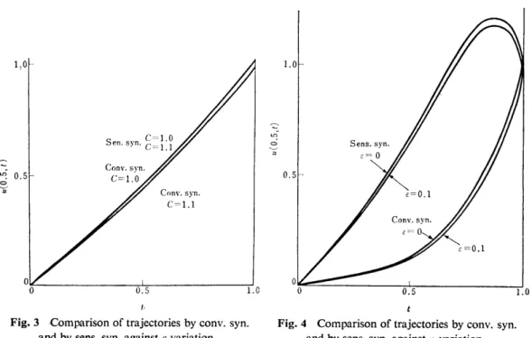
Numerical results for a variable parameter c with its nominal value c.= 1.0 are shown in Fig. 3 where a==O.1, b=2.0, ki == k2=:1.0 and the actual value ofa parameter c is 1.1.
The optimal performance costs are O.191 for the conventional synthesis and O.143 for thc sensitivity synthesis. Fig. 3 also shows that the state trajectory for the sensitivity synthcsis does not depend on the variation of the parameter c.
(Example 5,2) j-variation
Consider the following time-delay game with a terminal constraint u(1, x)=sin nx:
Ou(t, x)10t :a02u(t, x)lax2+u(t-s, x)+bif(t, x)+b2g(t, x)
OÅqtÅq1, OÅqxÅq1 ti(t, A-)=O --6SlltfE{lO, u(t, O)=:u(t, 1)==•O,
J == ,•i, j6 .S 6(ktf2 - iÅq 2g2)dt dx.
Numerical results for the nominal value e, = O are shown in Fi' g. 4 where a=O.Ol, b=2.0, c=1.0 and ki= Ic2 =1.0. Fig. 4 shows the state trajectories at x=O.5 of both the actual
g.ystein (e=O.1) and the model system (s =O) corresponding to the conventional synthesis and the sensitivity synthesis with a sensitivity constraint z(1, x)=:O. The optimal perfor- mance costs are O,657 for the conventional synthesis and 1.333 for the sensitivity one.
6. Conclusions
The distributed parameter differential games and the sensitivity synthesis of optimal strategies for them have been discussed in this paper.
The differential games presented here also can be applied to make minimax synthesis for the optimal control problems of the system with unknown functions which may be in some sense large. Then the sensitivity games can be applied to compensate the violence of the state constraints against the parameter variations in some sense small.
The numerical resultf have shown that there is a possibility to reduce minimax per- formance costs by the sensitjvity synthesis, Moreover it has been shown that the sensi-
.
Two-Player Zerosum Distributed Parameter DiiTerential Gtmies and Sensitivity Synthesis 21
1.0
A
LC)tt
o' O.5
••
$•
o
Conv. .g. yn.
':';
o.
e p
1.0
O.5
Conv. syn.
b=-2.2
Conv.s.vn. b=2.0 Sens. g. vn. b=-2 O b ==•-2.2
o
O O.5 1.0i
Sens. syn. t
Fig. 1 Comparison of trajectories by conv, syn. Fig. 2 Comparison of trajectories by conv. syn.
and by sens. syn. against a-variation and by sens. syn. against b-variation
1,O
A
----n. O.5
vo.
cr
s.n. syn• S' ll-IIIIOI
Conv. 'svn.
C=1.0
Conv. syn.
C=:1,1
t-..