the Theory of Visosity Solutions
Shigeaki Koike
2nd edition
9 May 2013
MathematialInstitute, TohokuUniversity,Aoba,Sendai,Miyagi980-8578JAPAN
Thisbook wasoriginallywrittenin Japanese forundergraduate students
in the Department of Mathematis of Saitama University. In fat, the rst
hand-written draft was prepared for a series of letures on the visosity so-
lution theory forundergraduate students inEhimeUniversity andHokkaido
University.
The aimhere is topresent a briefintrodutionto the theory of visosity
solutionsforstudentswhohaveknowledgeonAdvaned Calulus(i:e:dier-
entiation and integration on funtions of several-variables) and hopefully, a
littleonLebesgue Integration and Funtional Analysis. Sine this is written
for undergraduate students who are not neessarily exellent, I try to give
\easy" proofs throughout this book. Thus, if you do not feel any diÆulty
to read User's guide [6℄, youshould try toread that one.
Ialsotry not onlytoshow thevisosity solutiontheory but alsotomen-
tion some related \lassial"results.
Our plan of this book is as follows: We begin with our motivation in
setion 1. Setion 2introdues the denition of visosity solutionsand their
properties. In setion 3, we rst show \lassial"omparison priniples and
then, extend them to visosity solutions of rst- and seond-order PDEs,
separately. We establish two kindsof existene results via Perron's method
and representation formulas for Bellmanand Isaas equationsin setion 4.
Wedisuss boundary value problems forvisosity solutionsinsetions5.
Setion6isashortintrodutiontotheL p
-visositysolutiontheory,onwhih
we have anexellent book [4℄.
In Appendix, whih is the hardest part, we give proofs of fundamental
propositions.
In orderto learn more onvisosity solutions,I givea listof \books":
Apopularsurveypaper[6℄byCrandall-Ishii-Lionsonthetheoryofvisos-
ity solutions of seond-order, degenerate ellipti PDEs is stilla good hoie
for undergraduate students to learn rst. However, to my experiene, it
seems a bithard for average undergraduate students tounderstand.
Bardi-CapuzzoDoletta'sbook[1℄ontainslotsofinformationonvisos-
itysolutionsforrst-orderPDEs(Hamilton-Jaobiequations)whileFleming-
Soner's [10℄ omplements topis on seond-order (degenerate) ellipti PDEs
with appliations instohasti ontrol problems.
Barles' book [2℄ is also nie to learn his original tehniques and Frenh
language simultaneously !
visosity solutions in the near future, whih must be more advaned than
this.
For an important appliation via the visosity solution theory, we refer
to Giga's [12℄ onurvatureow equations. Also, I reommend the readerto
onsult LetureNotes [3℄(Bardi-Crandall-Evans-Soner-Souganidis)not only
for various appliations but also for a \friendly" introdution by Crandall,
whorstintroduedthenotionofvisositysolutionswithP.-L.Lionsinearly
80s.
If the reader is interested in setion 6, I reommend him/her to attak
Caarelli-Cabre's [4℄.
As ageneral PDE theory, althoughthere are so many bookson PDEs, I
only referto my favorite ones; Gilbarg-Trudinger's[13℄and Evans' [8℄. Also
as atextbook forundergraduate students, Han-Lin'sshort leturenotes [14℄
is a good hoie.
Sine this is a text-book, we do not refer the reader to original papers
unless those are not mentioned inthe books in our referenes.
Aknowledgment
Firstof all,I wouldliketo expressmythanks toProfessors H. Morimoto
andY.Tonegawaforgivingmetheopportunitytohaveaseriesofleturesin
theiruniversities. IwouldalsoliketothankProfessorsK.Ishii,T.Nagasawa,
andagraduatestudent,K.Nakagawa,fortheirsuggestionsonthe rstdraft.
I wish toexpress my gratitude to Professor H. Ishii for havinggiven me
enormous supply of ideas sine 1980.
I alsowish to thank the reviewerfor several important suggestions.
MynalthanksgotoProfessorT.Ozawaforreommendingmetopublish
thismanusript. HekindlysuggestedmetohangetheoriginalJapanesetitle
(\A seret lub onvisosity solutions").
AlthoughI orretedmanyerrorsinthe rstversion,theremust besome
mistakes in this version. I would be glad if the reader would kindly inform
me errorsand typos et.
IwouldliketothankT.Imai,H.Ishii,K.Ishii,K.Kohsaka,H.Mitake,T.
Nagasawa,S.Nakagawa,T. Nozokido,M.Ohta,andT.Ohtsukaforpointing
out numerous errors inthe rst edition.
9 May 2013 Shigeaki Koike
1 Introdution 1
1.1 From lassial solutionsto weak solutions 2
1.2 Typial examplesof weak solutions 4
1.2.1 Burgers' equation 4
1.2.2 Hamilton-Jaobi equation 6
2 Denition 9
2.1 Vanishingvisosity method 9
2.2 Equivalent denitions 17
3 Comparison priniple 23
3.1 Classial omparison priniple 24
3.1.1 Degenerate elliptiPDEs 24
3.1.2 UniformlyelliptiPDEs 24
3.2 Comparison priniplefor rst-order PDEs 26
3.3 Extension to seond-order PDEs 31
3.3.1 Degenerate elliptiPDEs 33
3.3.2 Remarkson thestrutureondition 35
3.3.3 UniformlyelliptiPDEs 38
4 Existene results 40
4.1 Perron'smethod 40
4.2 Representation formulas 45
4.2.1 Bellmanequation 46
4.2.2 Isaas equation 51
4.3 Stability 58
5 Generalized boundary value problems 62
5.1 Dirihlet problem 65
5.2 State onstraint problem 68
5.3 Neumann problem 72
5.4 Growth ondition at jxj!1 75
6 L -visosity solutions 78
6.1 A brief history 78
6.2 Denition and basi fats 81
6.3 Harnak inequality 84
6.3.1 Lineargrowth 85
6.3.2 Quadratigrowth 87
6.4 Holder ontinuity estimates 89
6.5 Existene result 92
7 Appendix 95
7.1 Proof of Ishii's lemma 95
7.2 Proof of the ABP maximum priniple 100
7.3 Proof of existene results for Pui equations 105
7.4 Proof of the weakHarnak inequlity 108
7.5 Proof of the loalmaximum priniple 113
Referenes 118
Notation Index 120
Index 121
Throughout this book, we will work in (exept in setions 4.2 and 5.4),
where
R
n
is open and bounded.
We denote by h;i the standard inner produt in R n
, and set jxj =
q
hx;xi for x 2 R n
. We use the standard notion of open balls: For r > 0
and x2R n
,
B
r
(x):=fy2R n
j jx yj<rg; and B
r :=B
r (0):
Fora funtion u: !R, we denote itsgradient and Hessian matrix at
x2, respetively, by
Du(x):=
0
B
B
B
u(x)
x
1
.
.
.
u(x)
xn 1
C
C
C
A
;
D 2
u(x):=
0
B
B
B
B
B
B
B
B
B
B
2
u(x)
x 2
1
j-th
2
u(x)
x
1 x
n
.
.
.
.
.
.
.
.
.
i-th
2
u(x)
x
i x
j
.
.
.
.
.
.
.
.
.
.
.
.
2
u(x)
xnx1
2
u(x)
x 2
n 1
C
C
C
C
C
C
C
C
C
C
A :
Also, S n
denotes the set of all real-valued nn symmetri matries. Note
that if u2C 2
(), then D 2
u(x)2S n
for x2.
We reall the standard orderingin S n
:
X Y () hX;ihY;i for 8 2R n
:
We will also use the following notion in setions 6 and 7: For = t
(
1
;:::;
n
), = t
(
1
;:::;
n ) 2 R
n
, we denote by the n n matrix
whose (i;j)-entry is
i
j
for 1i;j n;
=
0
B
B
B
B
B
B
B
B
1
1
j-th
1
n
.
.
.
.
.
.
.
.
.
i-th
i
j
.
.
.
.
.
.
.
.
.
.
.
.
n
1
n
n 1
C
C
C
C
C
C
C
C
A :
(PDEs for short):
F(x;u(x);Du(x);D 2
u(x))=0 in : (1:1)
We suppose (exept inseveral setions) that
F :RR n
S n
! R is ontinuous
with respet to allvariables.
1.1 From lassial solutions to weak solutions
As the rst exampleof PDEs, we present the Laplae equation:
4u=0 in: (1:2)
Here, we dene 4u:=trae(D 2
u). In the literature of the visositysolution
theory, we prefer tohave the minussign infront of 4.
Of ourse, sine we donot require any boundary ondition yet, all poly-
nomialsofdegreeone are solutionsof (1.2). Inmany textbooks(partiularly
thoseforengineers),underertainboundaryondition,welearnhowtosolve
(1.2) when has some speial shapessuh as ubes, balls, the half-spae or
the whole spaeR n
. Here, \solve"means thatwe ndanexpliit formulaof
u using elementary funtionssuh as polynomials,trigonometri ones,et.
However, the study on (1.2) in suh speial domains is not appliable
beause, for instane, solutions of equation (1.2) represent the density of a
gas ina bottle, whih is neithera ballnor a ube.
Unfortunately,ingeneraldomains,itseemsimpossibletondformulasfor
solutionsu withelementaryfuntions. Moreover, inorder toover problems
arisinginphysis,engineeringandnane,wewillhavetostudymoregeneral
and ompliatedPDEsthan(1.2). Thus, wehave todeal withgeneralPDEs
(1.1) in generaldomains.
Ifwegiveup havingformulasforsolutionsof(1.1),howdoweinvestigate
PDEs(1.1)? Inotherwords, whatistherightquestioninthestudyofPDEs
?
In the literature of the PDE theory, the most basi questions are as fol-
lows:
(2) Uniqueness: Is it the only solution ?
(3) Stability: If the PDE hanges a little,
does the solution hange a little ?
The importane of the existene of solutions is trivial sine, otherwise,
the study onthe PDE ould beuseless.
To explain the signiane of the uniqueness of solutions, let us remem-
ber the reason why we study the PDE. Usually, we disuss PDEs or their
solutions to understand some spei phenomena in nature, engineerings or
eonomis et. Partiularly, people working in appliations want to know
how the solution looks like, moves, behaves et. For this purpose, it might
be powerful to use numerial omputations. However, numerial analysis
only shows us an \approximate" shapes, movements, et. Thus, if there
are more than one solution, we do not know whih is approximated by the
numerialsolution.
Also,ifthe stabilityofsolutionsfails,weouldnotpreditwhatwillhap-
penfromthe numerialexperimentseven thoughthe uniquenessof solutions
holds true.
Now, let usome bak to the most essential question:
What is the \solution" of a PDE ?
For example, it is natural to all a funtion u : ! R a solution of
(1.1) if there exist the rst and seond derivatives, Du(x) and D 2
u(x), for
all x2, and (1.1) issatised ateah x2when we plug them inthe left
hand side of (1.1). Suh a funtion u willbe alled a lassial solution of
(1.1).
However, unfortunately, it is diÆult to seek for a lassial solution be-
ausewehavetoverifythatitissuÆientlydierentiableandthatitsatises
the equality (1.1) simultaneously.
Instead of ndingalassial solutiondiretly,wehave deided tohoose
the following strategy:
(A) Find a andidate of the lassial solution,
(B) Chek the dierentiability of the andidate.
In the standard books, the andidate of a lassial solution is alled a
weaksolution;iftheweaksolutionhastherstandseondderivatives,then
of solutions isalled the study onthe regularityof those.
Thus, with these terminologies, we may rewrite the above with mathe-
matial terms:
(A) Existene of weak solutions,
(B) Regularity of weak solutions.
However, when we annot expet lassial solutions of a PDE to exist,
what is the right andidate of solutions?
We will all a funtion the andidate of solutions of a PDE if it is a
\unique" and \stable" weak solution under a suitable setting. In setion 2,
we willdene suh aandidate named\visosity solutions"for a large lass
of PDEs, and in the proeeding setions, we will extend the denition to
more general (possibly disontinuous) funtions and PDEs.
In the next subsetion, we show a brief history on \weak solutions" to
remind what wasknown before the birth of visosity solutions.
1.2 Typial examples of weak solutions
In thissubsetion,wegivetwotypialexamplesof PDEstoderivetwokinds
of weak solutionswhih are unique and stable.
1.2.1 Burgers' equation
We onsider Burgers' equation,whih is amodelPDE in FluidMehanis:
u
t +
1
2 (u
2
)
x
=0 inR(0;1) (1:3)
under the initialondition:
u(x;0)=g(x) for x2R; (1:4)
where g isa given funtion.
In general, we annot nd lassial solutions of (1.3)-(1.4) even if g is
smooth enough. See [8℄for instane.
In order to look for the appropriate notion of weak solutions, we rst
introduea funtion spae C 1
0
(R[0;1))as a \test funtionspae":
C 1
0
(R[0;1)):=
(
2C 1
(R[0;1))
there is K >0 suh that
supp [ K;K℄[0;K℄ )
:
supp :=f(x;t)2R[0;1)j (x;t)6=0g:
Suppose that u satises (1.3). Multiplying (1.3) by 2 C 1
0
(R[0;1))
and then, using integration by parts, we have
Z
R Z
1
0 u
t +
u 2
2
x
!
(x;t)dtdx+ Z
R
u(x;0)(x;0)dx=0:
Sine there are no derivativesof u in the above, this equality makes sense if
u2[
K>0 L
1
(( K;K)(0;K)). Hene,wemayadaptthefollowingproperty
as the denition of weak solutionsof (1.3)-(1.4).
8
>
>
>
<
>
>
>
: Z
R Z
1
0 u
t +
u 2
2
x
!
(x;t)dtdx+ Z
R
g(x)(x;0)dx=0
for all 2C 1
0
(R[0;1)):
We often all this a weak solutioninthe distributionsense. As you no-
tied, we derive this notion by an essential use of integration by parts. We
say that a PDE is in divergene form when we an adapt the notion of
weak solutionsinthe distributionsense. Whenthe PDE isnotindivergene
form, wesay that itis in nondivergene form.
Wenotethat thesolutionof(1.3)mayhavesingularitieseven thoughthe
initialvalue g belongstoC 1
by anobservation via\harateristimethod".
From the denition of weak solutions, we an derive the so-alled Rankine-
Hugoniot ondition onthe set of singularities.
Ontheotherhand,unfortunately,weannotshowtheuniquenessofweak
solutions of (1.3)-(1.4) in general while we know the famous Lax-Oleinik
formula(see [8℄for instane), whihis the \expeted" solution.
Inordertoobtaintheuniqueness ofweaksolutions,forthe denition,we
add the following property (alled \entropy ondition") whih holds for the
expeted solution given by the Lax-Oleinik formula: There is C > 0 suh
that
u(x+z;t) u(x;t) Cz
t
for all(x;t;z)2R(0;1)(0;1). We allu anentropy solutionof (1.3)
if it is a weak solution satisfyingthis inequality. It is also known that suh
a weak solutionhas aertain stability property.
tant properties; \existene, uniqueness and stability". Thus, it must be a
right denition for weaksolutions of (1.3)-(1.4).
1.2.2 Hamilton-Jaobi equations
Next, we shall onsider general Hamilton-Jaobi equations, whih arise in
Optimal Control and ClassialMehanis:
u
t
+H(Du)=0 in(x;t)2R n
(0;1) (1:5)
under the same initialondition (1.4).
In this example,we suppose that H :R n
!Ris onvex, i:e:
H(p+(1 )q)H(p)+(1 )H(q) (1:6)
for allp;q 2R n
; 2[0;1℄.
Remark.SineaonvexfuntionisloallyLipshitzontinuousingeneral,
we do not need toassume the ontinuity of H.
Example.In Classial Mehanis,weoften allthis H a \Hamiltonian".
As asimple example of H,we have H(p)=jpj 2
.
Notiethat we annotadapt the weaksolutionin the distributionsense
for (1.5) sine we annot use the integration by parts.
We next introduethe Lagrangian L:R n
!R dened by
L(q)= sup
p2R n
fhp;qi H(p)g:
When H(p)=jpj 2
, it is easy to verify that the maximum is attained in the
right hand side of the above.
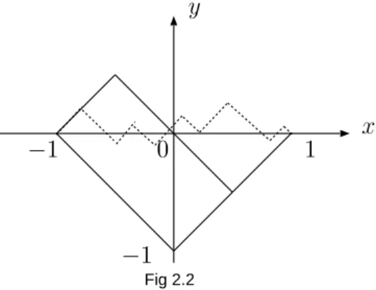
It is surprising that we have a neat formula for the expeted solution
(alled Hopf-Lax formula) presented by
u(x;t)= min
y2R n
tL
x y
t
+g(y)
: (1:7)
More preisely, it is shown that the right hand side of (1.7) is dierentiable
and satises (1.5) almost everywhere.
almost everywhere. However, if wedeide to use this notion asa weak solu-
tion, the uniqueness of those fails ingeneral. We willsee anexample in the
next setion.
As was shown for Burgers' equation, in order to say that the \unique
weak" solution is given by (1.7), we have to add one more property for the
denition of weak solutions: There is C >0 suhthat
u(x+z;t) 2u(x;t)+u(x z;t)Cjzj 2
(1:8)
for allx;z 2R;t>0. This isalled the \semi-onavity" of u.
We note that (1.8) is a hypothesis on the one-sided bound of seond
derivatives of funtionsu.
In 60s, Kruzkov showed that the limitfuntion of approximate solutions
by the vanishing visosity method (see the next setion) has this property
(1.8) when H is onvex. He named u a\generalized" solutionof (1.5) when
it satises (1.5) almosteverywhere and (1.8).
To my knowledge, between Kruzkov's works and the birth of visosity
solutions,there had been nobigprogress inthe study of rst-order PDEsin
nondivergene form.
Remark. The onvexity (1.6) is a natural hypothesis when we onsider
only optimal ontrol problems where one person intends to minimize some
\osts" (\energy"in termsof Physis). However, when we treatgame prob-
lems (one person wants to minimizeosts while the other tries tomaximize
them), we meet non-onvex and non-onave(i:e: \fully nonlinear")
Hamiltonians. See setion4.2.
In this book, sine we are onerned with visosity solutions of PDEs in
nondivergene form,for whih the integration by parts argument annot be
used todenethe notionofweaksolutionsinthedistributionsense, weshall
givetypialexamples of suh PDEs.
Example.(Bellman and Isaas equations)
We rst give Bellman equations and Isaas equations, whih arise in
(stohasti) optimal ontrol problems and dierential games, respetively.
As willbeseen, those are extensions of linear PDEs.
Let A and B be sets of parameters. For instane, we suppose A and B
are (ompat) subsets in R m
(for some m 1). For a 2 A, b 2 B, x 2 ,