Coupled finite-element/boundary-element analysis of a reciprocating self-excited induction generator in a harmonic domain

(1)

analysis of a reciprocating self‑excited induction generator in a harmonic domain

著者 Faiz J., Rezaeealam B., Yamada Sotoshi journal or

publication title

IEEE Transactions on Magnetics

volume 41

number 11

page range 4250‑4255

year 2005‑11‑01

URL http://hdl.handle.net/2297/6911

doi: 10.1109/TMAG.2005.855326

(2)

4250 IEEE TRANSACTIONS ON MAGNETICS, VOL. 41, NO. 11, NOVEMBER 2005

Coupled Finite-Element/Boundary-Element Analysis of a Reciprocating Self-Excited Induction

Generator in a Harmonic Domain

Jawad Faiz

¹

, Senior Member, IEEE, Behrooz Rezaeealam

¹

, and Sotoshi Yamada

²

, Member, IEEE

Center of Excellence on Applied Electromagnetic Systems, Department of Electrical and Computer Engineering,

Faculty of Engineering, University of Tehran, Tehran, Iran

Division of Biological Measurement and Applications, Institute of Nature and Environmental Technology (K-INET), Kanazawa University, Kanazawa 920-8667, Japan

This paper suggests a general method for analysis of a reciprocating self-excited induction generator based on the coupled finite- element/boundary-element method in a harmonic domain. The finite-element method is used for iron and copper parts in order to deal with nonlinearity and eddy currents, while the boundary-element method is utilized for the air-gap region between the moving parts using a free-space Green function that facilitates the application of a linear time periodic movement. The proposed method leads to a static global matrix that is symmetrical for particular boundary conditions. The results agree well with those obtained by the time- stepping methods.

Index Terms—Coupled finite-element/boundary-element method, harmonic balance method, reciprocating self-excited induction generator.

I. INTRODUCTION

I

NDUCTION generators are inexpensive and have no separate excitation; they can operate for a long period with no particular maintenance. Therefore, self-excited induction generators (SEIGs) can supply electrical power of an area far from the power system transmission lines and where nonconventional energies such as wind energy are available. However, SEIGs have their own disadvantages, including large dependency of the output voltage on the generator speed and load and the stator terminal capacitance requirement, which requires accounting for the speed and load variations. The models that are used for analysis of the SEIG are classified into two major groups. In the first group, a per phase equivalent circuit is utilized; in this case, the nodal-admittance method or loop-impedance method is used to establish the relationships of the machine-related parameters such as load, speed, and capacitance [1]. The second group uses the model; other equations, expressing the dependency between the steady-state parameters of the machine, are obtained using the harmonic balance method [2], [3]. In the above-mentioned methods, an attempt has been made to solve a nonlinear equation by an iterative procedure, where the experimental magnetization inductance versus magnetization current are available.

In this paper, a reciprocating SEIG with tubular structure, as shown in Fig. 1, is proposed. The SEIG is applicable in a free-piston generator system that is a combination of a linear engine and linear alternator. It is used in hybrid vehicles because this combination is compact, light, and very reliable [4], [5]. It has and windings, shunt exciting capacitances , and

Digital Object Identifier 10.1109/TMAG.2005.855326

resistive loads. Its model is nonlinear because of magnetic saturation, longitudinal end-effect, and unbalanced winding distri- bution that make the model difficult to deal with by analytical methods; thus, numerical methods are employed for its analysis.

A transverse edge effect does not exist due to the cylindrical construction.

This paper uses the coupled finite-element/boundary-element (FE–BE) method in harmonic domain for modeling a reciprocating SEIG [6]. Iron and copper parts of the generator are modeled by the FE method; therefore, the nonlinearity and eddy currents are taken into account. The air-gap region between the moving parts is modeled by the BE method using the free-space Green function. This method is especially suitable when a linear motion is involved in the electromagnetic devices to uncouple the moving and the stationary meshes. Here, the method is extended to the time periodic movement. For the particular case of a two-dimensional (2-D) coupled FE–BE model of a linear machine, it only requires elementary manipulations of the Green function and its normal derivative over a fundamental period.

In this manner, the SEIG model equations using time-stepping numerical methods is converted to the matrix form of the static coupled FE–BE equations, where they are used to obtain the state variables of the steady-state operation.

The proposed method leads to a static global matrix that is symmetrical for particular boundary conditions. However, this symmetry does not hold, in general, for the BE method. The results agree well with those obtained by time-stepping coupled FE–BE and FE methods.

II. COUPLEDFE–BE METHOD INHARMONICDOMAIN

WITHMOVEMENT

A. FE Regions

The primary and secondary domains were meshed using three-node triangular finite elements as shown in Fig. 2. The

(3)

Fig. 1. Reciprocating SEIG and equivalent circuits ofdandqwindings.

Fig. 2. Mesh of system.

equations are obtained using the Galerkin method. If F denotes the finite element region, based on the equivalent circuits of Fig. 1, the coupled field-circuit matrix equation of the proposed reciprocating SEIG (RSEIG) is as follows [7]–[9]:

(1)

is the magnetic potential and

is its normal derivative for those elements which have a side shared with the exterior domain . The exterior domain is broadened to lie outside the magnetic iron core and is the reluctivity of the air. and are the electromotive forces and terminal voltages of the windings

and , respectively.

is the stiffness sparse symmetrical matrix, is the damping symmetrical matrix due to eddy currents, and are the matrices for taking into account the forcing current densities and in the primary windings, as shown in

Fig. 1, . takes the exterior

domain into account, and is obtained as differential expressions of using matrices and . Circuit equations

are incorporated using matrices and with a nodal method [8].

B. BE Equations

The BE method is applied to the air gap that connects the primary and secondary domains [7], [8], [10]. This linear region with constant magnetic permeability is geometri- cally approximated by three-node boundary elements extracted from the primary and secondary element meshes. The contri- bution of all boundary elements to the magnetic field at a load point , in terms of the magnetic vector potential, is given by

(2)

(3)

(4) and are the nodal values of magnetic vector potential and its normal derivative, respectively. is the boundary factor and is the linear shape function between

(4)

each of the two adjacent boundary elements. is the Green function in axisymmetric coordinates

(5) and are complete elliptic integrals of the first and second kind, respectively, and the derivative is either or , according to the observation point [11].

The application of this formulation to all boundary nodes, using a collocation method, generates a BE system of equations. The values of the magnetic vector potential and its normal derivative on the nodes are unknowns

(6) The general expressions for and are as follows:

if if

(7) (8) where and denote the normal derivatives and

and correspond to the mutual effects of the boundary elements of primary ( ) and secondary ( ), when one of the load or field points is placed on the primary boundary and the other one is placed on the secondary boundary. Movement causes

and to be time variable as the distance varies with displacement. Similarly, the same holds for

and .

A combination of (1) and (6) gives the following coupled equations of the model:

(9)

where the continuity of the quantities and has been considered

(10)

C. Harmonic Balance

The periodic time variation of variables is approximated by a truncated Fourier series with frequency and period , where is the fundamental frequency of the reciprocating motion. Considering as nonzero harmonics, the corresponding

time-basis functions are

(11) The harmonic time discretization of and can thus be written as [12]

(12) The harmonic balance (HB) system of algebraic equations can be obtained by using the harmonic basis functions as weighting functions as well. Considering system of (7) results in

(13)

The application of the time discretization leads to the following system of equations:

(14)

where are the vectors of harmonic co-

efficients. If denotes a pair of harmonic functions, then (15) (16) (17) (18) (19) (20) (21) (22)

(5)

and so on for and that have diagonal block structure because of the orthonormality of the basis functions. Also

(23) (24) (25) and so on, for and that are full matrices because they require integration over a fundamental period of movement and needs to be considered iron saturation.

To maintain the symmetry of the matrices, particular atten-

tion must be paid to matrices .

is required because of the differential expressions

and .

D. Creating Symmetrical Matrix Equations and Applying Newton–Raphson Iteration

The last row of matrix (14), which is related to the boundary element equations, allows us to obtain a relationship between the nodal values of and on as follows:

(26) Rewriting this expression in the matrix equation of the first row in (14) and creating a new stiffness matrix , the system to be solved is

(27)

For simplicity, the Neumann condition and Dirichlet condition are applied to the boundaries in Fig. 2. These assumptions do not have a considerable effect on the results, as will be shown in comparison with time-stepping FE method. In this case, by considering (7) and (8), it can be proved that the BE matrices in (6) are symmetrical ( and ) because

is equal to on the boundaries , so the final matrix in the coupled system in (27) is symmetrical. However, this symmetry does not hold, in general, for the BE method.

Nonlinearity of the magnetic core causes the element stiffness matrix to be unknown and must be determined iter- atively. In [13], the Newton–Raphson method has been adopted in the FE-HB method using a differential reluctivity tensor that is applied to (27)

Jacobian Residual (28)

where is the incremental vector of

at the th iteration. Also, and

are evaluated for the th approximate solution, using the analytical equation of the magnetic saturation curve of the iron and , respectively.

Fig. 3. Time variation of main winding voltage during self-excitation process of generator.

Fig. 4. Steady-state terminal voltages.

III. RESULTS

The proposed method for SEIGs is applied to the reciprocating generator of Fig. 1. The generator has a tubular structure in which the secondary (translator) has been slotted to reduce the effective air gap, instead of a smooth top cap layer of copper.

The secondary length is twice the primary length, and the primary length is equal to the stroke length. The primary has two separate windings which constitute a two-phase structure and each slot has one coil with 120 turns.

Taking into account the mass of the translator, the imposed motion profile of the secondary is assumed to be:

meters and the maximum relative speed to be 10 m/s. The proposed SEIG for free-piston generator application has a higher reciprocating frequency compared to the permanent magnet counterparts (25–30 Hz) [4], [5], because the majority of the translator mass of the permanent magnet-type generator belongs to the magnets, which leads to the reduction of the reciprocating frequency compared with the proposed induction type.

The fundamental period of movement is subdivided into 92 time steps to calculate the integrations (24–25) in the motion-

dependant entries of and . The

model is also simulated by a time-stepping hybrid FE–BE solver [7], [10]. Fig. 3 shows the voltage build up as the main winding voltage . Self-excitation of the generator begins either by a residual air-gap flux or charge on the excitation capacitors.

This residual flux-linkage induces voltage in the primary windings when the translator moves. With sufficient capacitance, the process continues leading to the increase of induced primary voltages and until it settles down to a steady-state op- erating condition determined by the air-gap flux saturation. The steady-state results are shown in Fig. 4 for main ( ) and auxiliary

(6)

Fig. 5. Instantaneous magnetic flux lines of generator.

Fig. 6. Spectrum of voltagesU andU .

Fig. 7. Harmonic components of the flux lines of HB3: (a) first component, (b) second component, (c) third component, and (d) fourth component.

( ) voltages , and its instantaneous magnetic flux dis- tribution has been shown in Fig. 5. The spectrum of the terminal voltages is depicted in Fig. 6, where the fundamental frequency is 39.7 Hz.

Three HB simulations are carried out. The spectrum of these three simulations based on the HB, denoted as HB1, HB2, and HB3, is as follows: HB1: 0, 1 HB2: 0, 1, 2, and HB3: 0, 1, 2, 3, 4. The flux patterns for the HB3 simulation are shown in Fig. 7.

The third harmonic is concentrated around the air gap.

The HB results for are shown in Fig. 8, where harmonic components 0, 39.7, 79.4, 119.1, and 158.8 Hz are taken into

Fig. 8. Waveform of voltageU obtained with HB1, HB2, HB3, and time stepping.

Fig. 9. Mesh for time-stepping pure FE method.

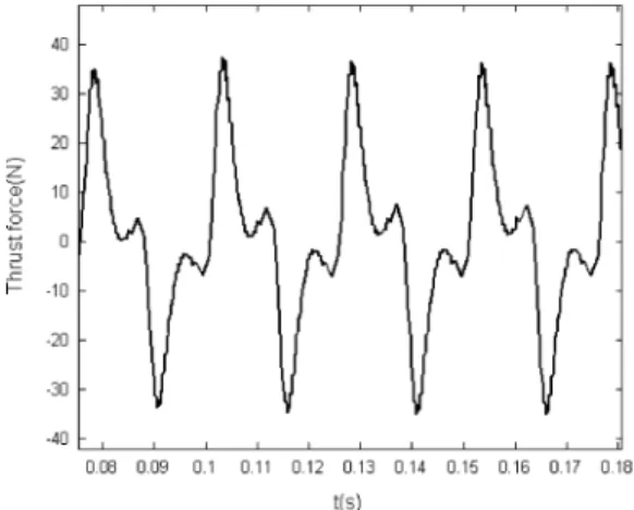
Fig. 10. Waveform of thrust force between primary and secondary parts.

account. The HB results for steady-state operation are closely identical to the time-stepping methods, including the transient coupled FE–BE method and transient FE method. The mesh for time-stepping pure FE is depicted in Fig. 9, [14] and the results for time-stepping FE and time-stepping coupled FE–BE at steady state are identical as shown in Fig. 8.

The required computation time, however, is very long for the transient period; it depends on the exciting capacitance, and sometimes it is longer than 6 h. For a similar situation, it lasts approximately 3 h and 20 min for time-stepping FE, 1 h and 30 min for the time-stepping coupled FE–BE method, and 15 min for the HB3 method. This indicates the benefits of the HB method over the time-stepping methods. In the coupled FE–BE method, the whole mesh includes 1280 elements and 977 nodes, while the air-gap region is treated by the BE method.

For transient FE simulation, the whole mesh includes 1800 elements and 1548 nodes. In comparison with the FE method, the coupled FE–BE method reduces the dimensions of the

(7)

Fig. 11. Peak of thrust force versus capacitance.

Fig. 12. Effective value of output voltages versus capacitance.

system matrices and avoids dominant changes in the global stiffness matrix at each time step because of geometry changes.

The waveform of the thrust force between the primary and secondary parts has been depicted in Fig. 10, which shows a pulsed power due to the reciprocating linear motion.

For different exciting capacitances, the fundamental frequency does not vary, because it is determined by the fundamental frequency of the imposed motion profile. As the exciting capacitance increases, the saturation level increases, and the peak value of the thrust force increases as shown in Fig. 11.

As a result, the output voltages and , and thus output power, increase. A variation of versus has been plotted in Fig. 12. There is no self-excitation where the capacitance is smaller than or larger than and voltage de-excitation occurs [2].

IV. CONCLUSION

The calculation procedure for the coupled FE–BE method combined with HB method has been presented and extended to include time-periodic movement. It has been suggested for steady-state analysis of a reciprocating SEIG. The proposed numerical method provides a straightforward procedure for the analysis of the self-excited systems. To analyze the SEIG, only the magnetization characteristic of the iron is required, while the analytical methods require an experimental magnetization inductance curve (versus magnetization current). This could be

helpful in the design of an SEIG and reluctance generator that need Ferro-resonance phenomenon to stabilize the self-excitation. Although the proposed numerical method is more compli- cated than the analytical ones, it can accurately deal with magnetic core saturation.

For the 2-D case of a linear machine with linear time-periodic movement, it only requires elementary manipulations of the Green function and its normal derivative. For particular boundary conditions, the static global matrix is symmetrical.

The results obtained by the proposed numerical method and that of time-stepping FE and coupled FE–BE methods has been compared, which shows a favorable computing time for the proposed method to acquire the steady-state solution.

REFERENCES

[1] T. F. Chan, “Analysis of self-excited induction generators using an iteration method,”IEEE Trans. Energy Convers., vol. 10, no. 3, pp. 502–506, Sep. 1995.

[2] O. Ojo, “Minimum airgap flux linkage requirement for self-excitation in stand-alone induction generator,”IEEE Trans. Energy Convers., vol. 10, no. 3, pp. 484–492, Sep. 1995.

[3] J. Chen, “Nonlinear transient and steady state analysis for self-excited single-phase synchronous reluctance generator,” dissertation collection, West Virginia Univ., Morgantown, 2001.

[4] W. R. Cawthorne, P. Famouri, J. Chen, N. N. Clark, T. I. McDaniel, R.

J. Atkinson, S. Nandkumar, C. M. Atkinson, and S. Petreanu, “Devel- opment of a linear alternator-engine for hybrid electric vehicle applications,”IEEE Trans. Veh. Technol., vol. 48, no. 5, pp. 1797–1802, Oct.

1999.

[5] W. M. Arshad, P. Thelin, T. Backstrom, and C. Sadarangani, “Use of transverse-flux machines in a free-piston generator,”IEEE Trans. Ind.

Appl., vol. 40, no. 5, pp. 1092–1100, Oct. 2004.

[6] R. Pascal, P. Conraux, and J.-M. Bergheau, “Coupling between finite elements and boundary elements for the numerical simulation of induction heating processes using a harmonic balance method,”IEEE Trans.

Magn., vol. 39, no. 3, pp. 1535–1538, May 2003.

[7] L. Pichon and A. Razek, “Hybrid finite-element method and boundary- element method using time-stepping for eddy-current calculation in axisymmetric problems,”Proc. Inst. Elect. Eng., pt. A, vol. 136, no. 4, pp.

217–222, Jul. 1989.

[8] W. N. Fu, P. Zhou, D. Lin, S. Stanton, and Z. J. Cendes, “Modeling of solid conductors in two-dimensional transient finite-element analysis and its application to electric machines,”IEEE Trans. Magn., vol. 40, no. 2, pp. 426–434, Mar. 2004.

[9] C. A. Brebbia,The Boundary Element Method for Engineers. London, U.K.: Pentech, 1978.

[10] L. Pichon and A. Razek, “Force calculation in axisymmetric induction devices using a hybrid FEM-BEM technique,”IEEE Trans. Magn., vol.

26, no. 2, pp. 1050–1053, Mar. 1990.

[11] A. Stratton,Electromagnetic Theory. New York: McGraw-Hill, 1941.

[12] J. Gyselinck, L. Vandevelde, P. Dular, C. Geuzaine, and W. Llegros, “A general method for the frequency domain FE modeling of rotating electromagnetic devices,”IEEE Trans. Magn., vol. 39, no. 3, pp. 1147–1150, May 2003.

[13] J. Gyselinck, P. Dular, C. Geuzaine, and W. Legros, “Harmonic balance finite element modeling of electromagnetic devices: A novel approach,”

IEEE Trans. Magn., vol. 38, no. 2, pp. 521–524, Mar. 2002.

[14] M. Jarnieux, D. Grenier, and G. Meunier, “FEM computation of eddy current and forces in moving systems application to linear induction launcher,”IEEE Trans. Magn., vol. 29, no. 2, pp. 1989–1992, Mar. 1993.

Manuscript received February 26, 2005; revised July 16, 2005.

(8)

Jawad Faiz(M’90-SM’93) received the Ph.D degree in electrical engineering from the University of Newcastle upon Tyne, U.K., in 1988.

He is now a Professor and the Director of Center of Excellence on Applied Electromagnetic Systems at the Department of Electrical and Computer Engi- neering, University of Tehran, Tehran, Iran. His teaching and research interests are switched reluctance and variable reluctance motors design and design and modeling of electrical machines, drives, and transformers.

Dr. Faiz is a member of the Iran Academy of Sciences.

Behrooz Rezaeealamreceived the B.Sc. degree in electronics engineering from Isfahan University of Technology and the M.Sc. degree in control engineering from the University of Tehran, Tehran, Iran, in 1997 and 2000, respectively. He is currently pursuing the Ph.D degree from the University of Tehran.

His research subjects are induction generators, linear induction machines, finite-element modeling, and control of electrical drives.

Sotoshi Yamada(M’86) received the Dr. Eng. degree from Kyushu University, Fukuoka, Japan, in 1985.

He is now a Professor at the Institute of Nature and Environmental Engi- neering, Kanazawa University, Kanazawa, Japan. He has been engaged in research on nondestructive testing by giant-magnetoresistance sensor, power magnetic devices, numerical electromagnetic field calculation, and biomagnetics.

Dr. Yamada is a member of the Institute of Electrical Engineers of Japan, the Magnetics Society of Japan, Japan AEM Society, and Japan Biomagnetism and Bioelectromagnetics Society.