Numerical methods for 1-D hyperbolic-type problems with free boundary
Faizal M
AKHRUS∗, Yoshiho A
KAGAWA, Alvi S
YAHRINI Graduate School of Natural Science and Technology, Kanazawa University, Kakuma, Kanazawa, 920–1192, Japan (Received June 29, 2015 and accepted in revised form August 31, 2015)Abstract We study a 1-D hyperbolic-type problem with free boundary which describes the motion of a piece of tape being peeled off from a surface. The graph of the solution represents the shape of the tape, which displays contact angle dynamics at the free bound- ary (the location of peeling). The contact angle dynamics lead to singularities located on the free boundary, which cause a slight difficulty. Under some assumptions, this problem can be solved numerically by a so-called fixed domain method. This method is a numer- ical method which transforms the domain of the positive part of the solution into a fixed domain using a change of variables and solves the problem in that domain. Although this method has a high accuracy, it can not be applied in some cases. Hence other numer- ical methods are chosen for solving a regularized problem, i.e., the singularities on the free boundary are regularized by a smoothing function. The numerical methods are: two types of finite difference methods, the finite element method and discrete Morse flow. In this paper, the error of solving the regularized problem instead of the original problem is calculated. Since the choice of the parameter for smoothing function is important for the accuracy, we propose a formula to estimate the optimal parameter in order to mini- mize the error. This formula is verified by numerical experiments and we find that it can estimate the optimal parameter. In addition, based on comparisons between the numeri- cal methods, we find that the finite difference methods have better performance than the other methods.
Keywords. hyperbolic free boundary problem, fixed domain method, finite element method, discrete Morse flow
1 Introduction
In this paper we investigate numerical methods for solving a one-dimensional hyper- bolic-type problem with a free boundary. Our problem can be derived from a physical
∗Corresponding author. Current address: Department of Computer Science, Faculty of Mathemat- ics and Natural Sciences, Gadjah Mada University, Sekip Unit 3, Bulaksumur, Sleman, Indonesia.
e-mail: faizal [email protected]
model of a piece of tape which is attached to a surface and peeled off from the edge smoothly. Under certain assumptions [2], the motion of the tape is described by a stationary point of the following action integral in a suitable function space:
J ( u ) =
τ0
Ω
1
2 |∇ u |
2− 1
2 ( u
t)
2χu>0+ Q
22
χu>0
dxdt , (1.1)
where u : ( 0 ,τ) ×
Ω→
Ris a scalar function which represents the shape of the tape,
Ωis a domain in
Rd( d ≥ 1 ) , Q is the surface tension and
χu>0is a characteristic function of the set {(x,t) : u(x,t) > 0 } . The following Euler-Lagrange equation can be derived from functional (1.1) under certain assumptions [2]:
u
tt=
Δuin (Ω × ( 0 ,
τ))∩ {u > 0 },
|∇ u |
2− ( u
t)
2= Q
2on (Ω× ( 0 ,τ )) ∩
∂{ u > 0 }. (1.2) When d = 1, under certain conditions, [3] showed that the existence and the uniqueness of its solutions are obtained locally.
On the other hand, we derive the following equation from (1.2) (see Section 2):
χ{u>0}
u
tt=
Δu− Q
2| Du |
Hd∂ {u > 0} in
Ω× (0,τ), (1.3) where
Hdis the d-dimensional Hausdroff measure and Du =
∂
u
∂
x
1,...,
∂u
∂
x
d,
∂u
∂
t
. Next, we consider the following equation as the regularized problem of (1.3)
χ{u>0}
u
tt=
Δu − Q
22 (χ
ε)
( u ) in
Ω× ( 0 ,
τ),(1.4) where
χε(u) ∈ C
∞(R) is a smoothing of the characteristic function such that (χ
ε)
≥ 0 and
χε
( u ) =
0 u ≤ 0 , 1 u ≥
ε.The main purpose of this paper is to investigate the error obtained in solving (1.4) utilizing several numerical methods. The error is obtained by comparing with the solution of (1.2) which is equivalent to the original problem (1.3) if the solution is non-negative. We solve (1.2) by the fixed domain method. This method has high accuracy [2]. Therefore we use its solution to calculate the error, and from this error, we know that the choice of parameter
εis important to the accuracy. Therefore we propose a formula to get the optimal
εand confirm that this formula applies based on our experiments. We discuss this in Section 4.1–4.2.
The numerical methods that we use are:
1. explicit method 1 (spatial central difference + time forward difference)
2. explicit method 2 (spatial and time central difference) 3. finite element method (FEM)
4. discrete Morse flow (DMF).
We choose explicit method 1 and 2 as they are standard methods. Here, explicit method 2 is a standard finite difference method which can be used to analyze the error of the solution of the regularized problem. We choose FEM as it is widely used to approx- imate solutions of hyperbolic problems and DMF is chosen since it is used in many hyperbolic-type problems with constraints [1]. We conduct the comparisons of these numerical methods in Section 4.4.
The second purpose of this paper is to investigate the effectivity of different kinds of smoothed characteristic functions. We consider two types of smoothed characteristic functions and compare them to get the suitable one (see Section 4.3). The last purpose is to implement more advanced case such as a model in which there are more than one free boundary points that appear or vanish during the simulation (see Section 4.5).
2 Derivation of (1.3)
This section depends on [4]. We show the derivation of (1.3). Let Q
T: =
Ω×(0 ,τ ) . We assume u ∈ H
2({ u > 0 }) ∩ C ( Q
T) is a nonnegative solution of (1.2) such that contact set { u > 0 } has a sufficiently regular boundary and { u > 0 } ⊂ C
0,1. By definition
(u
tt−
Δu)(ϕ) = −
QT
{u
tϕt−
∇u·∇ϕ}dxdt, where u
tt−
Δu is a measure. Since u is nonnegative,
χ{u>0}
u
tt( E ) =
E∩{u>0}
u
tt= u
ttE ∩ { u > 0 }
= u
tt(E),
where E ⊂ Q
T. Thus
χ{u>0}u
tt= u
ttin the measure sense. Then, by using the above assumptions, we can calculate
χ{u>0}
u
tt−
Δu
(ϕ) = −
QT
{ u
tϕt−
∇u ·
∇ϕ} dxdt
=
{u>0}
( u
tt−
Δu )ϕ dxdt −
∂{u>0}
|∇ u |
2− ( u
t)
2| Du |
ϕd
Hm= −
∂{u>0}
Q
2| Du |
ϕd
Hm,
and directly obtain (1.3).
3 Numerical Methods
From this section throughout this paper, we assume that
Ωis 1-dimensional. This section explains our numerical methods. Let us introduce some notations. The domain
Ωis divided into N intervals, x
0< x
1< ··· < x
N, then the characteristic function is smoothed as follows
(χ
ε)
( u ) =
1 /ε 0 < u <
ε,0 otherwise . (3.1)
As we will show later in Section 4.3, the smoothness of
χεdoes not significantly influence accuracy, and therefore to speed up the numerical computations we use a smoothing function
χεas above that is only Lipschitz continuous. Next, the charac- teristic function is
χ{u>0}
( x
i, t ) =
1 if max ( u ( x
i−1, t ), u ( x
i, t ), u ( x
i+1, t )) > 0 , 0 otherwise
and
χε
( u ) =
u0
(χ
ε)
( s ) ds .
At last, since we are interested in observing the biggest error of the solutions during time t, we define the error of numerical solutions as
E
u= max
i=0,...,N k=0,...,M
| u
∗( x
i, t
k) − u
ki|,
where u
∗is the exact solution or fixed domain method solution and u
kiis the numerical solution at x
iin time t
k.
3.1 Fixed domain method (FDM)
For equation (1.2), we build the numerical solution as explained in [2]. We assume that the free boundary contains a single point l ( t ) . Here, u ( x , t ) is the solution at position x and time t, l ( t ) is the position of the boundary at time t and l
0= l ( 0 ) . Since the key of fixed domain method in this case is to solve only in {u > 0}, the coordinates are mapped using function
y = 2x l ( t ) − 1
and become ( 0 , l ( t )) × ( 0 ,τ ) ( x , t ) → ( y , t ) ∈ (− 1 , 1 ) × ( 0 ,
τ). Rewriting equation (1.2) using ( y , t ) , one has
u
tt− 4 − (( y + 1 ) l
( t ))
2l ( t )
2u
yy− 2 ( y + 1 ) l
( t )
l ( t ) u
ty− ( y + 1 ) l ( t ) l
( t ) − 2 ( l
( t ))
2l ( t )
2u
y= 0
in (− 1 , 1 ) × ( 0 ,τ ) and
l
( t ) = ±
1 −
Ql ( t ) 2u
y( 1 ,t)
2
,
where l
( t ) ≥ 0. Now, the y-space [− 1 , 1 ] is discretized into ˜ N equal intervals and we can get the following equations
d
dt u
i( t ) = v
i( t ), (3.2)
d
dt v
i(t) = 4 − ((y
i+ 1 )l
(t))
2l ( t )
2u
i+1(t) − 2u
i(t) + u
i−1(t) (Δ y )
2+ 2 ( y
i+ 1 ) l
( t ) l ( t )
v
i+1( t ) − v
i−1( t ) 2
Δy + ( y
i+ 1 ) l ( t ) l
( t ) − 2 ( l
( t ))
2l ( t )
2u
i+1( t ) − u
i−1( t )
2
Δy , i = 1 ,..., N ˜ − 1 , (3.3) l
( t ) = ±
1 −
Ql ( t ) 2u
Ny( t )
2
. (3.4)
We solve (3.2)–(3.4) using the 4
th-order Runge-Kutta method.
3.2 Explicit method 1 (spatial central difference and time forward dif- ference)
We represent equation (1.4) using an explicit method with u
xxapproximated by central differencing. Suppose u
t= v then
d
dt u
i(t) = v
i(t), (3.5)
d
dt v
i( t ) = u
i−1( t ) − 2u
i( t ) + u
i+1( t ) (Δ x )
2− Q
22 (χ
ε)
( u
i( t )), if
χ{u>0}( x
i, t ) = 1 , (3.6) v
i( t ) = 0 , if
χ{u>0}( x
i, t ) = 0 , (3.7) where i = 1 ,..., N − 1. We solve (3.5)–(3.7) using the 4
thorder Runge-Kutta.
3.3 Explicit method 2 (spatial and time central difference)
This method utilizes a standard finite difference discretization. We approximate u
xxand u
ttfrom equation (1.4) using centered differencing. Here, [ 0 ,τ ] is divided into M equal intervals, 0 = t
0< t
1< ··· < t
M=
τ, so we have
χ{u>0}
( x
i, t
k) u
ki+1− 2u
ki+ u
ki−1(Δ t )
2= u
ki+1− 2u
ki+ u
ki−1(Δ x )
2− Q
22 (χ
ε)
( u
ki),
i = 1 ,..., N − 1 and k = 1 ,..., M − 1 ,
where u
ki= u(x
i,t
k) . Then we calculate the solutions using the following
⎧⎪
⎪⎪
⎪⎨
⎪⎪
⎪⎪
⎩
u
ki+1= 2u
ki− u
ki−1+(Δ t )
2u
ki+1− 2u
ki+ u
ki−1(Δ x )
2− Q
22 (χ
ε)
( u
ki)
, if
χ{u>0}( x
i, t
k) = 1 , u
ki+1= 0 , if
χ{u>0}( x
i, t
k) = 0 .
(3.8)
3.4 Finite Element Method
To implement finite element method, we multiply equation (1.4) by any test function
ξ∈ C
0∞(Ω) and integrate over the space domain
Ω
(χ
{u>0}u
tt− u
xx+ Q
22 (χ
ε)
(u))ξ dx = 0 . By integration by parts we obtain
Ω
(χ
{u>0}u
ttξ+ u
xξx+ Q
22 (χ
ε)
( u )ξ ) dx = 0 , ∀ξ ∈ C
0∞(Ω). (3.9) We divide
Ωinto N intervals and find the approximate solution of (3.9) in the set
V
t= {u ∈ C
0(
Ω)¯ : u|
∂Ω= f (·,t), u is linear on every [x
k−1, x
k], k = 1 ,..., N}
for each time t ∈ ( 0 ,
τ), where f : ¯
Ω×[ 0 ,τ ] is a given function. Then the approximate solution can be described by u ( x , t ) =
∑Ni=0a
i( t )ϕ
i( x ) , where
ϕi
( x ) =
1 − | x − x
i|
Δx
+
, i = 0 ,..., N .
Here the symbol ( )
+implies ( f ( x ))
+= max ( f ( x ), 0 ) . We substitute the approximate solution u to (3.9)
Ω
χ{u>0}
∑
N i=0a
iϕiξ+ ∑
Ni=0
a
iϕiξ+ Q
22 (χ
ε)
∑
Ni=0
a
iϕiξdx = r , ∀ξ ∈ C
0∞(Ω), (3.10) where r is the residual which comes from the approximated representation of function u. We choose
ϕj, j = 1 ,..., N − 1, as our test function and rewrite (3.10) as follows:
∑
N i=0
a
i
Ωχ{u>0}ϕiϕj
dx
+ ∑
Ni=0
a
i
Ωϕiϕj
dx
+ Q
22
Ω
(χ
ε)
∑
Ni=0
a
iϕiϕjdx = 0 , j = 1,2,. . . ,N-1.
This can be written in a vector form
Ba
+ Aa + Q
22 C ( a ) = p ,
where a is the column vector with entries a
1,..., a
N−1,
A = 1
Δx
⎡
⎢⎢
⎢⎢
⎢⎣
2 − 1 0 0 0 ··· 0 0
− 1 2 − 1 0 0 ··· 0 0
0 − 1 2 − 1 0 ··· 0 0
.. . .. . .. . .. . .. . .. . . .. ...
0 0 0 0 0 ··· − 1 2
⎤
⎥⎥
⎥⎥
⎥⎦
and
B =
Δx6
⎡
⎢⎢
⎢⎢
⎢⎣
4 ˜
χ( a
1)
χ˜ ( a
1) 0 0 0 ··· 0 0
χ˜ ( a
2) 4 ˜
χ( a
2)
χ(˜ a
2) 0 0 ··· 0 0 0
χ˜ ( a
3) 4 ˜
χ(a
3)
χ(˜ a
3) 0 ··· 0 0 .. . .. . .. . .. . .. . .. . . .. .. . 0 0 0 0 0 ···
χ(˜ a
N−1) 4 ˜
χ(a
N−1)
⎤
⎥⎥
⎥⎥
⎥⎦
.
Here, ˜
χ( a
i) = 1 , whenever max ( a
i−1, a
i, a
i+1) is greater than zero and ˜
χ(a
i) = 0 oth- erwise. Here, C is a column vector whose elements are determined by a and p is determined by boundary values.
We approximate a
using central difference with a
ki= a
i( t
k) and a
k=( a
k1,..., a
kN−1) : B a
k+1− 2a
k+ a
k−1(Δ t )
2+ Aa
k+ Q
22 C ( a
k) = p . The final form is
Ba
k+1= 2Ba
k− Ba
k−1− (Δt)
2Aa
k+ Q
22 C(a
k) − p
. (3.11)
We define a
ki+1= 0 , if b
ii= 0 where b
iiis the diagonal element of matrix B at i
throw.
In general, matrix B is non-symmetric. We can change the position of the known value of a
ki+1to the right hand side and adjust the matrix B to be a symmetric matrix. Now, we approximate the solution a
k+1of (3.11) by conjugate gradient method.
3.5 Discrete Morse Flow
Let us consider problem (1.4) with u
0as the initial value, v
0as the initial velocity and u
1= u
0+
Δtv
0. Now, we determine the time step
Δt =
τ/ M, where M > 0 is a natural number. Then, the approximate solution for the next time t = k
Δt, k = 2 , 3 ,..., M is defined by the minimizer u
k∈
Kof
J
k( u ) =
Ω
| u − 2u
k−1+ u
k−2|
22 (Δ t )
2 χ{u>0}dx + 1 2
Ω
|∇ u |
2dx + Q
22
Ωχε
( u ) dx ,
where u
j(x)= u(x,t
j), t
j= jΔt ( j =k− 2 , k− 1 ) and
K= {u ∈
W1,2(Ω) ;u = g on
∂Ω}.We approximate u
kas a piecewise linear function, so that the functional’s values are approximated:
J
k(u) ≈ ∑
Ni=1
xi
xi−1
| u − 2u
k−1+ u
k−2|
22 (Δ t )
2 χ{u>0}+ 1
2 |∇u|
2+ Q
22
χε(u)
dx. (3.12) We calculate the first term as follows:
xi
xi−1
|u − 2u
k−1+ u
k−2|
22 (Δ t )
2 χ{u>0}dx
=
⎧⎪
⎪⎪
⎪⎪
⎪⎪
⎨
⎪⎪
⎪⎪
⎪⎪
⎪⎩
( v
2+ w
2+ vw )
Δx
6 (Δt)
2u
i−1> 0 , u
i> 0 , ( w
2+ ( v
2)
2+ wv
2) x
c− x
i6 (Δ t )
2u
i−1≤ 0 , u
i> 0 , (( w
2)
2+ v
2+ w
2v ) x
c− x
i−16 (Δ t )
2u
i−1> 0 , u
i≤ 0 ,
0 otherwise ,
where v = | u
i−1− 2u
ki−−11+ u
ki−−12| , w = | u
i− 2u
ki−1+ u
ki−2| , u
i−1= u ( x
i−1, t ) , u
i= u ( x
i, t ) , v
2= v − w − v
u
i− u
i−1u
i−1, w
2= v
2and x
c= x
i−1−
Δxu
i− u
i−1u
i−1. The second term is 1
2
xixi−1
|∇ u
i|
2dx = ( u
i+1− u
i)
22
Δx , and for the third term we have
xi
xi−1
χε
(u)dx
=
⎧⎪
⎪⎪
⎪⎪
⎪⎪
⎪⎪
⎪⎪
⎪⎪
⎪⎨
⎪⎪
⎪⎪
⎪⎪
⎪⎪
⎪⎪
⎪⎪
⎪⎪
⎩
Δ
x u
max≥
ε,u
min≥
ε,
1 −
Δx u
min− u
max− u
min( u
min−
ε)2ε − (ε − u
max)
u
max≥
ε,0 ≤ u
min<
ε, u
maxΔx
2 ( u
max− u
min) u
max≥
ε,u
min≤ 0 ,
Δx
2
ε( u
max+ u
min) 0 ≤ u
max<
ε,0 ≤ u
min<
ε, u
2maxΔx
2
ε(u
max− u
min) 0 ≤ u
max<
ε,u
min≤ 0 ,
0 otherwise ,
where u
max= max ( u
i−1, u
i) and u
min= min ( u
i−1, u
i) . We find the minimizer of (3.12)
using a non-linear conjugate gradient method.
4 Numerical results
In this section, we explain our experiments and the results. In our experiments we compare two problems. The first problem is
⎧⎪
⎪⎪
⎪⎪
⎪⎪
⎨
⎪⎪
⎪⎪
⎪⎪
⎪⎩
u
tt= u
xxin (Ω × ( 0 ,τ )) ∩ { u > 0 }, (u
x)
2− (u
t)
2= Q
2on (Ω × ( 0 ,τ )) ∩
∂{u > 0 }, u ( 0 , t ) = f ( t ),
u ( x , 0 ) = g ( x ), u
t( x , 0 ) = h ( x ),
approximated by the fixed domain method and the second problem is
⎧⎪
⎪⎪
⎪⎪
⎨
⎪⎪
⎪⎪
⎪⎩
χ{u>0}
u
tt= u
xx− Q
22 (χ
ε)
(u) in
Ω× ( 0 ,
τ),u(0,t) = f(t),
u ( x , 0 ) = g ( x ), u
t( x , 0 ) = h ( x ),
approximated by two types of finite different method, FEM or DMF. The initial con- ditions of our experiments are
l
0= 1 Q
2+ f
( 0 )
2, g ( x ) = max ( 1 − 1
l
0x , 0 ), h ( x ) =
f
( 0 ) 0 < x ≤ l
0, 0 l
0< x , and f (t) are as follows:
Case 1
Peeling speed is constant f ( t ) = at + 1. The exact solution of this case is u ( x , t ) = max ( 1 + t −
l10x , 0 ) .
Case 2
Peeling speed is increasing f (t) = (at + 1)
2.
Case 3Peeling speed is decreasing f ( t ) = √
at + 1.
Case 4
Peeling speed is stopping at some times f ( t ) = 1 + at + sin t
Case 5Peeling direction is downward (pasting the tape).
g ( x ) = max ( 10 − 1 l
0x , 0 ), f ( t ) = 10 − at ,
h ( x ) =
f
( 0 ) 0 < x ≤ l
0,
0 l
0< x .
Case 6
Peeling directions are upward and downward (oscillating tape) f(t) = 1 + 0 . 3 sint.
In addition, we construct the exact solution of (1.4) for a special case. Let
Ω=
R,then we describe problem (1.4) as
χ{u>0}
u
tt=
Δu − Q
22 (χ
ε)
( u ) in
R× ( 0 ,τ ). (4.1) Let u
ε: ( 0 ,τ ) ×
R→
Rbe the exact solution of (4.1) and we assume that u
εis written as
u
ε(x,t) = F(z), z = x − vt,
where v is a constant and 0 < v < 1, F :
R→
R;F (0) = 0, F
(0) = 0, F ∈ C
1,1(R).
This solution can be considered as peeling tape with constant peeling speed, where the solution is increasing but keeps its shape. Therefore we get
χ{F>0}
v
2F
( z ) = F
( z ) − Q
22 (χ
ε)
( F ). (4.2)
We separate F into three intervals { F ≥
ε},{ 0 < F <
ε} and { F = 0 } . We assume that the free boundary point is at z = 0 ( F ( 0 ) = 0 ) and z = z
ε( F ( z
ε) =
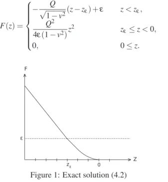
ε) as shown in Figure 1. Then we can construct the exact solution as follows
F ( z ) =
⎧⎪
⎪⎪
⎪⎨
⎪⎪
⎪⎪
⎩
− Q
√ 1 − v
2( z − z
ε) +
εz < z
ε, Q
24
ε( 1 − v
2) z
2z
ε≤ z < 0 ,
0 , 0 ≤ z .
(4.3)
Figure 1: Exact solution (4.2)
4.1 Error in the peeling tape model using smoothed characteristic func- tions
We solve cases 1–6 using explicit method 2 and compare with the exact solution for case 1 and the fixed domain method solutions for cases 2–6. The parameters are shown in Table 1 below.
Table 1: Parameters for explicit method 2 and fixed domain method
Q
2 Ωa
Δt
Δx
explicit method 2 1 [0, 15] 1 0.9Δx varied fixed domain method 1 [− 1 , 1 ] 1 0.0005625 0.002
The comparisons are shown in Figure 2. From the figures, we can see that the errors of solutions for all cases tend to be small when
Δx is decreasing with
ε. They show that small and big
εgive large error and so we analyze this error pattern. Since the precise error is difficult to find, we only approximate it. Here, the error of the explicit method 2 satisfies the inequality
i=
max
0,...,N k=0,...,M| u
∗( x
i, t
k) − u
ki| ≤ E
1+ E
2,
where
E
1= max
i=0,...,N k=0,...,M
| u
∗( x
i, t
k) − u
ε( x
i, t
k)|, E
2= max
i=0,...,N k=0,...,M
| u
ε( x
i, t
k) − u
ki|
and u
∗is the exact solution of problem (1.2), u
εis the exact solution of (1.4) and u is the solution of (3.8). From this inequality we expect to obtain the error pattern.
We calculate the error of finite difference (explicit method 2). We define e
ki= u
ε( x
i, t
k−1) − 2u
ε( x
i, t
k) + u
ε( x
i, t
k+1)
Δ
t
2− u
ε( x
i−1, t
k) − 2u
ε( x
i, t
k) + u
ε( x
i+1, t
k)
Δx
2+ Q
22 (χ
ε)
( u
ε( x
i, t
k)) (4.4)
and subtract (4.4) from (4.1) to obtain u
εtt− u
εxx+ Q
22 (χ
ε)
( u
ε) = u
ε( x
i, t
k−1) − 2u
ε( x
i, t
k) + u
ε( x
i, t
k+1)
Δt2− u
ε( x
i−1, t
k) − 2u
ε( x
i, t
k) + u
ε( x
i+1, t
k)
Δx
2+ Q
22 (χ
ε)
( u
ε( x
i, t
k)) − e
ki. Since the error occurs near z = 0 and z
ε, at first we calculate for z = 0 (x
i− vt
k= 0 ) .
e
ki= F ( v
Δt ) − 2F ( 0 ) + F (− v
Δt )
Δ
t
2− u
tt− F (−Δ x ) − 2F ( 0 ) + F (Δ x )
Δx
2+ u
xx.
(a)Euat timeτ=9 in case 1 (b)Euat timeτ=9 in case 2
(c)Euat timeτ=9 in case 3 (d)Euat timeτ=9 in case 4
(e)Euat timeτ=9 in case 5 (f)Euat timeτ=7 in case 6
Figure 2: The errors of explicit method 2 for cases 1–6 Since we want to find the upper bound of the error, we note
e
ki≤
F ( v
Δt ) − 2F ( 0 ) + F (− v
Δt )
Δt
2− u
tt+
− F (−Δ x ) − 2F ( 0 ) + F (Δ x )
Δx
2+ u
xx
≤
− Q
2v
24
ε( 1 − v
2)
+
Q
24
ε(1 − v
2)
.
Since 0 < v < 1, we have
e
ki≤ Q
22
ε(1 − v
2) .
In the same way, we can get the estimate of e
kifor z
ε, which is also less than or equal to Q
22
ε( 1 − v
2) . Since | e
ki| is the error of the finite differencing, we expect E
2∼ g
2uΔx2
ε, (4.5)
where g
uis the norm of the gradient of the solution and g
2u= Q
21 − v
2. In this experiment, we can consider the gradient is a constant C.
Next, we assume the error E
1= C ˜
ε. Therefore the total error is
i=
max
0,...,N| u
∗( x
i, t
k) − u
ki| ≤ C ˜
ε+ C
Δx
ε
. (4.6)
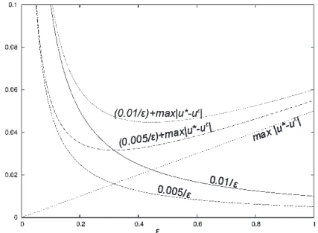
The graph of this total error can be seen in Figure 3. In this figure, there are two
Δx:
Figure 3: Estimation from above of the total error for explicit method 2
0.01 and 0.005. When
Δx decreases, the error also decreases for particular
ε. It also shows that when
εis big or small, the error increases. This is approximately similar to the error pattern in Figure 2a and serves to justify our results.
4.2 Comparisons of solution having different gradient
We are also interested in investigating the choice of
εto get optimal error related to the
gradient of the solution near the free boundary point ( g
u) . The relation between g
uand
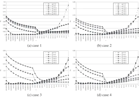
the error is shown in (4.5). The gradient of the solution is approximated by calculating
(a) case 1 (b) case 2
(c) case 3 (d) case 4
Figure 4: The errors of solution for case 1–4 with different gradient and
Δx = 0 . 000625 at
τ= 7
the linear regression of five u
iwhose values are nearest to the value 0 . 1. This value is chosen since, based on Figure 2a–2d, when
ε= 0 . 1, they display similar errors for different
Δx.
To see the relation between the error of the solutions and g
u, we conduct a few experiments using cases 1–4 with different g
u. We choose only cases 1–4 since they are enough to represent different kinds of solutions. We set the gradient of the solution at time
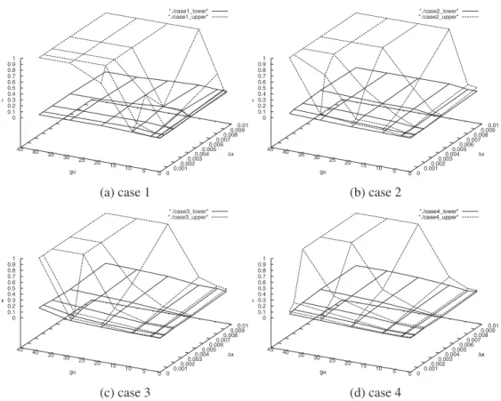
τ= 7 to be 1 to 40. The results are shown in Figures 4 and 5. Figure 4 shows that the range of optimal
εbecomes larger when g
uincreases. In addition, Figure 5 shows that there are two surfaces. The lower surfaces describe the lower bound of the range for the optimal
ε, while the upper surfaces describe the upper bound of the range for the optimal
ε. From the figure, the range of the optimal
εbecomes large if the gradient of the solution increases.
The optimal
εcan be derived from (4.6). Therefore we have
ε= Cg
u√
Δ
x . (4.7)
From the experiments above, the range of constant C in (4.7) is shown in Figure 6. In
this figure, each vertical line indicates the range of constant C which applies for the
gradient 1 to 40. It shows when the constant C is between 0.15–0.16, it satisfies for all
0 0.001 0.002 0.003 0.004 0.005 0.006 0.007 0.008 0.009 0.01 5 0
15 10 25 20 35 30 45 40 0 0.1 0.2 0.3 0.4 0.5 0.6 0.7 0.8 0.91
"./case1_lower"
"./case1_upper"
x gu
(a) case 1
0 0.001 0.002 0.003 0.004 0.005 0.006 0.007 0.008 0.009 0.01 5 0
15 10 25 20 35 30 45 40 0 0.1 0.2 0.3 0.4 0.5 0.6 0.7 0.8 0.91
"./case2_lower"
"./case2_upper"
x gu
(b) case 2
0 0.001 0.002 0.003 0.004 0.005 0.006 0.007 0.008 0.009 0.01 5 0
15 10 25 20 35 30 45 40 0 0.1 0.2 0.3 0.4 0.5 0.6 0.7 0.8 0.91
"./case3_lower"
"./case3_upper"
x gu
(c) case 3
0 0.001 0.002 0.003 0.004 0.005 0.006 0.007 0.008 0.009 0.01 5 0
15 10 25 20 35 30 45 40 0 0.1 0.2 0.3 0.4 0.5 0.6 0.7 0.8 0.91
"./case4_lower"
"./case4_upper"
x gu
(d) case 4
Figure 5: The lower and upper bound of optimal
εfor cases 1–4 at
τ= 7
Figure 6: The range of constant C for cases 1–4 with different
Δx
cases and
Δx. Therefore, we conclude that the constantC is approximately 0.15–0.16.
4.3 Comparisons of smoothed characteristic functions
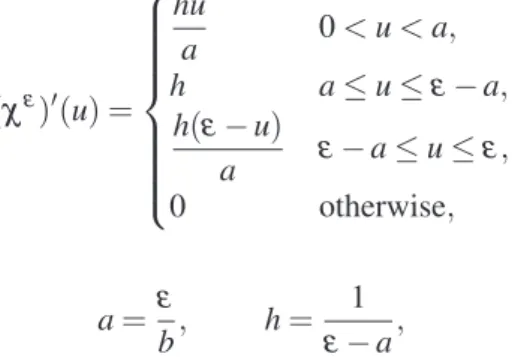
Here, we will compare two smoothed characteristic functions satisfying (3.1) and
(χ
ε)
(u) =
⎧⎪
⎪⎪
⎪⎪
⎪⎨
⎪⎪
⎪⎪
⎪⎪
⎩
hu
a 0 < u < a , h a ≤ u ≤
ε− a ,
h (ε − u )
a
ε− a ≤ u ≤
ε,0 otherwise ,
(4.8)
where
a =
εb , h = 1
ε− a ,
b is a positive number. Function (4.8) has smoother transitions than (3.1). We want to know whether smooth transitions influence the accuracy. The goal of this experiment is to get the appropriate smoothed characteristic function.
We apply these two functions in equation (1.4) with parameters Q
2= 1,
Ω= [ 0 , 15 ] , a = 1,
Δx = 0 . 005 and
Δt = 0 . 9
Δx and solve using explicit method 2. The errors for each case at time level
τ= 9 (case 6 uses
τ= 7) are shown in Figure 7. The errors are calculated using
E ˜
u= max
i=0,...,N k=0,...,M
| u
∗( x
i, t
k) − ( u
(3.1))
ki| or E ˜
u= max
i=0,...,N k=0,...,M