資料3－3　Physics Case for the 250 GeV Stage of the International Linear Collider（付日本語訳）

(1)

DESY-17-155

KEK Preprint 2017-31 LAL 17-059

SLAC–PUB–17161 October 2017

Physics Case for the 250 GeV Stage of the International Linear Collider

LCC Physics Working Group

Keisuke Fujii¹, Christophe Grojean^2,3, Michael E. Peskin⁴ (Conveners); Tim Barklow⁴, Yuanning Gao⁵, Shinya Kanemura⁶, Hyungdo Kim⁷, Jenny List², Mihoko Nojiri^1,8, Maxim Perelstein⁹, Roman P¨oschl¹⁰, J¨urgen Reuter², Frank Simon¹¹, Tomohiko Tanabe¹²,

James D. Wells¹³, Jaehoon Yu¹⁴; Mikael Berggren², Moritz Habermehl², Sunghoon Jung⁷, Robert Karl²,

Tomohisa Ogawa¹, Junping Tian¹²; James Brau¹⁵, Hitoshi Murayama^8,16,17 (ex officio)

ABSTRACT

The International Linear Collider is now proposed with a staged machine design, with the first stage at 250 GeV with a luminosity goal of 2 ab⁻¹. In this paper, we review the physics expectations for this machine.

These include precision measurements of Higgs boson couplings, searches for exotic Higgs decays, other searches for particles that decay with zero or small visible energy, and measurements ofe⁺e⁻annihilation toW⁺W⁻ and 2-fermion states with improved sensitivity. A summary table gives projections for the achievable levels of precision based on the latest full simulation studies.

arXiv:1710.07621v2 [hep-ex] 3 Nov 2017

資料３－３

(2)

1 High Energy Accelerator Research Organization (KEK), Tsukuba, Ibaraki, JAPAN

2 DESY, Notkestrasse 85, 22607 Hamburg, GERMANY

3 Institut f¨ur Physik, Humboldt-Universit¨at zu Berlin, 12489 Berlin, GERMANY

4 SLAC, Stanford University, Menlo Park, CA 94025, USA

5 Center for High Energy Physics, Tsinghua University, Beijing, CHINA

6 Department of Physics, Osaka University, Machikaneyama, Toyonaka, Osaka 560- 0043, JAPAN

7 Dept. of Physics and Astronomy, Seoul National Univ., Seoul 08826, KOREA

8 Kavli Institute for the Physics and Mathematics of the Universe, University of Tokyo, Kashiwa 277-8583, JAPAN

9 Laboratory for Elementary Particle Physics, Cornell University, Ithaca, NY 14853, USA

10 LAL, Centre Scientifique d’Orsay, Universit´e Paris-Sud, F-91898 Orsay CEDEX, FRANCE

11 Max-Planck-Institut f¨ur Physik, F¨ohringer Ring 6, 80805 Munich, GERMANY

12 ICEPP, University of Tokyo, Hongo, Bunkyo-ku, Tokyo, 113-0033, JAPAN

13 Michigan Center for Theoretical Physics, University of Michigan, Ann Arbor, MI 48109, USA

14 Department of Physics, University of Texas, Arlington, TX 76019, USA

15Center for High Energy Physics, University of Oregon, Eugene, Oregon 97403-1274, USA

16 Department of Physics, University of California, Berkeley, CA 94720, USA

17 Theoretical Physics Group, Lawrence Berkeley National Laboratory, Berkeley, CA 94720, USA

(3)

4.1 Basic observables: σ, σ·BR . . . 12 4.2 Expected precisions for Higgs boson couplings in the κ formalism . . 14 4.3 Expected precisions for Higgs boson couplings in the EFT formalism 15 4.4 Measurement of the Higgs boson mass and CP . . . 20 5 Comparison of the ILC capabilities for the Higgs boson to the pre-

dictions of new physics models 21

5.1 Models of electroweak symmetry breaking and the Higgs field . . . . 21 5.2 Comparisons of models to the ILC potential . . . 25

6 Invisible and exotic Higgs decays 27

7 Opportunities for discovering direct production of new particles 29

8 e⁺e⁻ →W⁺W⁻ at 250 GeV 31

9 Two-fermion production at 250 GeV 34

10 Program of the ILC beyond 250 GeV 36

11 Conclusions 38

A Projected ILC physics measurement uncertainties 40

(4)

(5)

1 Introduction

The International Linear Collider (ILC) is a linear electron-positron collider planned for physics exploration and precision measurements in the energy region of 200–

500 GeV. This report summarizes the expectations for measurements of the Higgs boson and searches for physics beyond the Standard Model in the program of this accelerator at 250 GeV in the center of mass.

The physics potential of the ILC is known to be very impressive. A detailed accounting of the expectations for this machine was presented in 2013 as a part of the ILC Technical Design Report [1,2] and in white papers prepared for the American Physical Society’s study of the future of US particle physics (Snowmass 2013) [3–6].

As the ILC experiments have been studied in more detail, our Working Group has published updated expectations for the general ILC program [7] and for the direct search for new particles at this collider [8].

In the past year, the program of the ILC has been reshaped in the expectation of an international agreement and start of construction. The Linear Collider Collaboration has recast the project as a staged program with the first stage at 250 GeV [9]. This would significantly lower the initial cost of the machine and provide a focused, nearer- term goal for the project. In this approach, the 250 GeV stage of the ILC needs to be justified on its own merit rather than as a part of a broader program that includes running at higher energies. At the same time, new studies have revealed a very strong physics potential for the 250 GeV stage of the ILC that was not specifically emphasized in the reports cited above. The purpose of this article is to summarize the case for the 250 GeV machine stage as it is understood today. We will see that there is a compelling physics case for the ILC that applies already at its 250 GeV stage.

Section 2 of this report updates the 2015 report on ILC operating scenarios [10], giving estimates of time vs. integrated luminosity for an ILC project with 250 GeV, top quark threshold, and 500 GeV stages.

The most important objective of a 250 GeV e⁺e⁻ collider is to make precision measurements of the couplings of the 125 GeV Higgs boson to vector bosons, quarks, and leptons. Unlike the situation at proton colliders, all of the major Standard Model decay modes of the Higgs boson will be individually identifiable ine⁺e⁻ experiments.

This means that it is possible to extract the absolute strengths of Higgs boson couplings to high precision in a model-independent analysis. In Sections 3 and 4 of this report, we will explain how this can be done and give projected errors for the coupling constant determinations.

The search for new physics beyond the Standard Model is probably the most important goal of particle physics today. The LHC experiments are carrying out

(6)

intensive searches for new particle of many types, and dark matter detection experiments add to the variety of searches. Because shifts of the Higgs couplings can be induced by mixing with or loop corrections from very heavy particles, the study of these couplings gives a route to new physics that is essentially orthogonal to these methods. Today, the LHC experiments are probing for large shifts of the Higgs couplings, but, in typical models, the shifts of the Higgs couplings from their Standard Model values are predicted to be small, at the 10% level and below. Thus, high- precision experiments, beyond the expectations for LHC, are needed. In our opinion, this precision study of the Higgs boson is the most important suggested probe for new physics beyond the Standard Model that is not currently being exploited. This gives special impetus to the construction of a new accelerator for precision Higgs studies.

Qualitatively different models of new physics predict different patterns of deviation from the Standard Model prediction. If the Higgs couplings can be measured individually with high precision, it is possible to read the pattern and obtain information on the properties of the new physics model. We will expand on this point and present some examples in Section 5.

The Higgs boson provides another possible window into new physics. Potentially, it is easy for the Higgs boson to couple to new particles with no Standard Model interactions, particles that might make up the dark matter or might otherwise be hidden from experiments that rely on other probes. We will review the ILC capabilities for the discovery of invisible and exotic Higgs decays in Section 6.

In Sections 7, 8, and 9, we will discuss the capabilities of a 250 GeV e⁺e⁻ collider beyond its program on the Higgs boson. Section 7 will review the reach of such a machine for observation of the direct pair production of dark matter particles and other particles difficult to detect at the LHC. In Section 8, we will discuss the new information that will be available from the precision study of e⁺e⁻ → W⁺W⁻. In Section 9, we will review the ability ofe⁺e⁻ annihilation to fermion-antifermion pairs at 250 GeV to probe for new boson resonances and quark and lepton substructure.

Finally, in Section 10, we will review very briefly the capabilities of the ILC, after an energy upgrade, for measurements at 350 GeV, 500 GeV, and higher energies.

Indeed, the infrastructure of the ILC will support a long future of experiments with e⁺e⁻ collisions that would build on the success of the first 250 GeV stage.

An appendix gives a table of the projected measurement errors for the most important parameters. We recommend that these are the numbers that should be used in discussions of the ILC physics prospects and in comparisons of the ILC with other proposed facilities.

(7)

years

0 5 10 15 20 25

integrated luminosities [fb] ⁰

1000 2000 3000 4000

Luminosity Upgrade

ILC, Scenario H-20 ECM = 250 GeV ECM = 350 GeV ECM = 500 GeV Integrated Luminosities [fb]

Figure 1: The nominal 20-year running program for the 500-GeV ILC [10].

2 Plan for ILC evolution and staging

Following the publication of the ILC Technical Design Report [1,2,11–13], a canon- ical operating scenario was defined for the ILC [10]. This operating scenario assumed the construction of a 500-GeV machine, which within a 20-year period would accumulate integrated luminosities of 4 ab⁻¹, 2 ab⁻¹ and 200 fb⁻¹ at center-of-mass energies of 500 GeV, 250 GeV and 350 GeV, respectively, with beam polarizations of ±80%

for the electron beam and ±30% for the positron beam. Figure 1 shows the time evolution of the data-taking envisioned in [10], starting with operation at 500 GeV.

There were three main physics reasons for starting at 500 GeV: first, the ability to use both of the major Higgs boson production processes e⁺e⁻ → Zh and e⁺e⁻ → ννh to measure Higgs couplings; second, the ability to begin precision measurements of the couplings of the top quark, including the direct measurement of the top-Yukawa coupling from tthproduction, and third, the ability to exploit the maximal discovery range for new particles.

Nevertheless, a very important part of the ILC physics program relies on data collected in its running at 250 GeV, which already yields a substantial sample of about half a million Higgs bosons tagged with recoilingZ bosons and subject to very small backgrounds. Using new analyses for reconstructing the various Higgs decay modes and a new, more powerful theoretical approach, to be described in Section 3, we realized that the 250 GeV program alone can already give powerful and model- independent constraints on the Higgs properties. Thus, a staging scenario with a long first stage at 250 GeV makes sense from the point of view of physics. The purpose of this paper is to present this argument in detail.

The detailed plan and accelerator design for the 250 GeV stage of the ILC is described in [9]. In this section, we will discuss the implications of this plan for the

(8)

running scenario and luminosity expectations.

Construction of a 250 GeV machine rather than the full 500 GeV machine does change the expectation for the instantaneous luminosity that can be assumed in 250 GeV running. The original running scenario (Fig. 1) relied on the availability of the full cryogenic and radio-frequency power of the 500-GeV machine in order to double the repetition rate from 5 to 10 Hz when operating at 250 GeV. This option is not available when only half of the power is installed in a minimal 250 GeV machine.

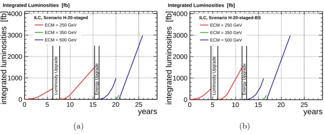
Therefore the total operating time for accumulating the same integrated luminosities as listed above stretches to 15 years of operation for the 250 GeV stage and to 26 years for the full ILC program. This luminosity evolution is shown in Fig. 2a.

There is a cost-neutral possibility to increase the instantaneous luminosity by fo- cussing the beam more strongly at the IP. This increases the level of beamstrahlung and e⁺e⁻ pair production. However, the ILC interaction region is designed to cope with operation at 500 GeV and even at 1 TeV. Since beamstrahlung is strongly energy- dependent, its effects at energies lower than these is much reduced, and so there is room for a more aggressive choice of beam parameters at 250 GeV. A revised set of accelerator parameters that implements this luminosity enhancement is presented in Section 5 of [9]. The effect of these new parameters on the run plan is illustrated in Fig. 2b. In this plan, the length of the 250 GeV stage is 11 years and the total operating time for the full program is only slightly longer than the original 20 years.

The exact effects of the new beam parameters on the detectors and the physics measurements, taking account of the new beam energy spectrum and pair background, still need to be evaluated quantitatively. All physics studies quoted in this document are performed with the TDR parameters and thus apply strictly speaking to the case shown in Fig. 2a. Nevertheless, we expect the differences to be small and are opti- mistic that similar results will be found with the new beam parameters corresponding to Fig. 2b.

It is well documented that beam polarization plays an essential role in the physics program of the ILC at higher energies [2]. As will be discussed in the following sections, the ability of the ILC to measure the dependence of cross sections on beam polarization is very important also for Higgs physics at 250 GeV. In [10], the fractions of integrated luminosity dedicated to each of the four possible sign combinations were proposed for each center-of-mass energy. For operation at 250 GeV, fractions of (67.5%, 22.5%, 5%, 5%) were forseen for (−+,+−,−−,++), where the first sign applies to the electron beam polarization and the second to that of the positron beam, giving emphasis to the−+ configuration as it has the largest Higgs production cross section. In our new theory framework, the left-right cross-section asymmetry plays an important role. To optimize the measurement of this quantity, we assume in this paper a sharing of (45%, 45%, 5%, 5%) among the various beam polarization choices.

(9)

years

0 5 10 15 20 25

integrated luminosities [fb] ⁰ 1000 2000 3000 4000

Luminosity Upgrade Energy Upgrade ILC, Scenario H-20-staged

ECM = 250 GeV ECM = 350 GeV ECM = 500 GeV Integrated Luminosities [fb]

(a)

years

0 5 10 15 20 25

integrated luminosities [fb] ⁰ 1000 2000 3000 4000

Luminosity Upgrade Energy Upgrade ILC, Scenario H-20-staged-BS

ECM = 250 GeV ECM = 350 GeV ECM = 500 GeV Integrated Luminosities [fb]

(b)

Figure 2: Run plan for the staged ILC starting with a 250-GeV machine under two different assumptions on the achievable instantaneous luminosity at 250 GeV. Both cases reach the same final integrated luminosities as in Fig. 1.

3 Effective Field Theory approach to precision measurements at e

⁺

e

⁻

colliders

The goal of the ILC program on the Higgs boson is to provide determinations of the various Higgs couplings that are both high-precision and model-independent.

It is easy to see how this can be achieved for some combinations of Higgs couplings.

In the reactione⁺e⁻→Zh, the Higgs boson is produced in association with aZ boson at a fixed lab-frame energy (110 GeV for√

s= 250 GeV). Up to small and calculable background frome⁺e⁻→ZZ plus radiation, observation of a Z boson at this energy tags the presence of a Higgs boson. Then the total cross section for e⁺e⁻ →Zh can be measured absolutely without reference to the Higgs boson decay mode, and the various branching ratios of the Higgs boson can be observed directly.

The difficulty comes when one wishes to obtain the absolute strength of each Higgs coupling. The coupling strength of the Higgs boson toAA can be obtained from the partial width Γ(h→AA), which is related to the branching ratio through

BR(h→AA) = Γ(h→AA)/Γ_h , (1) where Γ_his the total width of the Higgs boson. In the Standard Model (SM), the width of a 125 GeV Higgs boson is 4.1 MeV, a value too small to be measured directly from reaction kinematics. So the width of the Higgs boson must be determined indirectly, and this requires a model formalism.

In most of the literature on Higgs boson measurements ate⁺e⁻colliders, the width is determined using the κ parametrization. One assumes that the Higgs coupling to

(10)

each species Ais modified from the SM value by a mutiplicative factor κ_A. Then, for example,

Γ(h→ZZ^∗)

SM =κ²_Z , σ(e⁺e⁻→Zh)

SM =κ²_Z . (2)

where SM denotes the SM prediction. The e⁺e⁻ environment offers a sufficient number of measurements to determine all of the relevant parametersκ_A. In particular, the ratio

σ(e⁺e⁻→Zh)/BR(h→ZZ^∗) (3) is independent of κ_Z and directly yields the Higgs width. However, at the 250 GeV ILC even with 2 ab⁻¹ of data, the statistics to measureBR(h→ZZ^∗) is limited, and so the precision of the width determination is compromised. In the earlier literature, including [3,7], this problem was solved by using data from higher energies, making use of theW fusion reaction and the larger and more precisely measurable branching ratio BR(h→W W^∗).

There is a more serious problem with the κ formalism: It is not actually model- independent. In principle, the Higgs boson can have couplings to ZZ with two different structures,

δL = m²_Z

v (1 +η_Z)hZ_µZ^µ+ζ_Z1

vhZ_µνZ^µν . (4) Here the coefficients η_Z, ζ_Z represent independent corrections due to new physics effects.^∗ The Higgs boson coupling to W W has a similar structure, with parameters η_W, ζ_W. In the κ formalism, the couplings ζ_Z, ζ_W are assumed to be zero. The operator multiplying ζ_Z is momentum-dependent, so the effect of this term depends on the momentum configuration of the vector bosons. Indeed, for a 125 GeV Higgs boson and√

s = 250 GeV,

Γ(h→ZZ^∗)/SM = (1 + 2η_Z−0.50ζ_Z)

σ(e⁺e⁻ →Zh)/SM = (1 + 2η_Z+ 5.7ζ_Z). (5) Then the Z coupling information does not cancel out of (3) and so this ratio does not determine the Higgs width unambiguously.

There is an attractive solution to this problem. The fact that the LHC experiments have not yet observed new particles due to physics beyond the SM suggests that these particles are heavy, with masses above 500 GeV for electroweakly coupled states and above 1 TeV for strongly interacting states. If indeed new particles are sufficient heavy, we can describe the physics of the 125 GeV Higgs boson by integrating these particles out of the Lagrangian and replacing their effects by an expansion in operators

∗In principle, additional structures can be formed by making ηZ and ζZ functions of momentum. However, (4) is the most general structure that appears in the SM perturbed by dimension-6 operators only, a restriction that we will make below.

(11)

built of Standard Model fields. The SM itself is the most general gauge-invariant Lagrangian built of SM fields with operators of dimension up to 4. Corrections to the SM are then described by the addition of operators of dimension 6 and higher.

If the minimum mass of the new particles is M, operators of dimension 6 will have coefficients proportional to m²_h/M². These represent the first order in an expansion inm²_h/M². Possible operators of dimension 8 and higher are multiplied by additional factors of m²_h/M². It is then suggested to parametrize the effects of the most general new physics on the Higgs boson by writing an effective Lagrangian that consists of the SM Lagrangian plus the most general set of SU(3) ×SU(2) ×U(1)-invariant dimension-6 operators. This is called the Standard Model Effective Field Theory (EFT) formalism.

The EFT formalism has been accepted by the LHC community as the best way to parametrize deviations from the SM in Higgs physics and in vector boson interactions that might be observed at the LHC [14]. The advantage of this approach for the LHC experiments is that it provides a precise theoretical formalism in which radiative corrections can be computed. This is important at the LHC, because Higgs signatures often require suppressed decay modes with contributions from different basic couplings (for example, dileptons in the final state), and because quantitative predictions for QCD processes require NLO corrections. However, it is difficult to use this formalism in a completely general way at the LHC. The most important difficulty is that the the number of possible dimension 6 operators is very large. There are 59 dimension-6 operators that can be added to the SM Lagrangian even if we restrict ourselves to one generation of fermions and to baryon number-conserving operators. Most of these involve quark and gluon fields and are relevant to LHC reactions.

For reactions that involve only SM vector bosons, Higgs bosons, and light leptons, the number of possible operators is much smaller, though still sizable. In [15], it is argued that the most general effects of high-mass new physics on these reactions can be parametrized by 10 dimension-6 operators.^† The same 10 operators parametrize the new physics contributions to precision electroweak observables and to observables in e⁺e⁻ →W⁺W⁻. There are sufficient measurements available to an e⁺e⁻ collider to determine all 10 parameters without significant degeneracies. This gives a unified formalism for testing the SM, one that brings together the full set of measurements available at ane⁺e⁻collider. Inclusion of on-shell Higgs decays brings in 7 additional operators. Measurement of Higgs decays allows the coefficients of these additional operators to be determined also. Fits to prospective e⁺e⁻ collider data using the EFT formalism have been presented in [16–19]. The last of these papers emphasizes the completeness of the 17-parameter model and the ability to fit the 17 parameters simultaneously using the expected data set frome⁺e⁻ colliders.

†Of these 10 operators, 1 shifts the triple- and quadruple-Higgs couplings but does not affect single-Higgs processes at the tree level.

(12)

An illustration of the power of this formalism is given by the answer to the ques- tion posed at the beginning of this section. The problem, again, is that the hZZ and hW W couplings each involve two separate kinematic structures whose coefficients must be separately determined. The EFT formalism contains coefficients of dimension-6 operators that contribute to the η_Z,W and ζ_Z,W parameters defined in (4). However, theSU(2)×U(1)-invariance of the EFT Lagrangian leads to relations between the coefficients for Z and W. These relations are not simple, but they turn out to be very constraining. For the η parameters,

η_W =−1

2c_H + 2δm_W −δv η_Z =−1

2c_H + 2δm_Z−δv−c_T , (6)

where the c_i are coefficients of dimension-6 operators, δm_W, δv, and δm_Z are combinations of these coefficients that shift the parameters mW, GF, and mZ (and are constrained by the measured values of those quantities), and c_T is essentially the T parameter of precision electroweak formalism [20] and is constrained to be small by precision electroweak measurements. Similarly,

ζ_W = (8c_{W W})

ζ_Z = cos²θ_w(8c_{W W}) + 2 sin²θ_w(8c_{W B}) + (sin⁴θ_w/cos²θ_w)(8c_BB), (7) in which the parameters c_{W B}, c_BB also contribute to e⁺e⁻ →W⁺W⁻ and the Higgs decays to γγ and Zγ and so can be strongly constrained. The network of constraints essentially reduces the problem to be solved by ILC Higgs measurements to the determination of the two parametersc_H,c_{W W} using measurements of the process e⁺e⁻ → Zh and the decay h → W W^∗. For both reactions, there will be ample statistics at the 250 GeV ILC. A particular feature of interest is that new Higgs observables not previously considered in ILC studies become relevant. In particular, the polarization asymmetry and angular distributions in e⁺e⁻ →Zh turn out to put very strong constraints on ζ_Z orc_{W W} [19].

Remarkably, then, the EFT formalism, applied to the e⁺e⁻ world, realizes in a very beautiful way the hopes put forward by its proponents in the LHC world. It provides a single formalism that knits together constraints from precision electroweak measurements and from all of the processes, not only Higgs processes, that are measured in high-energy e⁺e⁻ reactions. The number of free parameters, describing the most general new physics perturbation, is large but manageable, and all relevant parameters can be determined independently. Although second-order electroweak corrections to already small perturbations are not obviously relevant, the formalism also provides a Lagrangian setting in which radiative corrections can be computed unambiguously. This formalism thus provides a powerful method for stringent tests of the SM and, we hope, discovery of new, beyond-SM effects.

(13)

4 Measurement of Higgs boson couplings

In the SM, all of the Higgs boson couplings are predicted in terms of the value of the mass of Higgs boson, which is now known to 0.2% accuracy at the LHC [21].

The observation of any deviation from these predictions would imply new physics beyond the Standard Model. As was already noted, and will be discussed further in Section 5, the expectations for deviations are small in typical BSM scenarios. It is thus one of the main goals for a futuree⁺e⁻ collider is to achieve O(1%) precision in the measurement of Higgs boson couplings. This goal has been demonstrated to be achievable at the ILC [2,3,7,10] for the running scenarios with a baseline of√

s= 500 GeV, based on full detector simulations for most of the observables.

Thus we focus here on the prospects for the measurement of Higgs boson couplings at the 250 GeV stage of ILC assuming a total integrated luminosity of 2 ab⁻¹.

In this section we will first introduce the basic observables that are used to fit for Higgs boson couplings. We will also discuss the expected precisions of branching ratios, which can be determined free of any theory assumptions. To quote absolutely normalized couplings, we need to determine the Higgs boson width, and this requires a theory framework. We will discuss the width determination in the κ and EFT formalisms described in the previous section, emphasizing the major consequences of the change from √

s = 500 GeV to 250 GeV and the new observables that play an important role in the EFT approach. Unless explicitly stated, all numbers shown in this section are for a total integrated luminosity of 2 ab⁻¹ and for beam polarization sharing as introduced in Section 2.

4.1 Basic observables: σ, σ·BR

The SM cross sections for the leading Higgs production processes in e⁺e⁻ annihilation with (P_e, P_p) = (−0.8,+0.3) polarized beams are shown in Fig.3. The process e⁺e⁻ →Zhattains its maximum cross section at√

s = 250 GeV, providing about half a million Zh events from an integrated luminosity of 2 ab⁻¹. This allows the precise measurement of the inclusive cross section σ_Zh, using the recoil mass technique, and of the ratesσ_Zh·BRfor various decay modes. Up-to-date estimates for measurements ofσ_Zh andσ_Zh·BRare given in the Appendix of [19]. Most notably,σ_Zh is measured to 1.0% for both (−+) and (+−) initial polarization states at √

s = 250 GeV. An example of the recoil mass distribution in the Z → µ⁺µ⁻ channel is given in Figure 4 (left).

With both σ_Zh and σ_Zh · BR measured, the absolute branching ratios can be determined independently of any fitting formula. Among the SM branching ratios, the best measured ones would be BRbb andBRτ τ, with accuracies of 0.89% and 1.4%

respectively. If there are O(1%) or larger exotic decay modes, a first hint would

(14)

Figure 3: Cross sections for the three major Higgs production processes as a function of center of mass energy, from [2].

(15)

already be provided by observing the resulting deviations in BR_bb and BR_{τ τ}. The branching ratiosBR_cc and BR_gg, which are very challenging to access directly at the LHC, can be measured to 3.2% and 2.7% respectively. BR_{W W} and BR_ZZ, which play a special role in the total width determination, can be measured to 1.9% and 6.7% respectively. The branching ratios to the rare decay modes,BR_γγ andBR_µµ are limited by available statistics and can be measured only to 13% and 27% respectively.^‡ However, these measurements can be improved by combination with LHC results, since the ratios of branching ratiosBR_ZZ/BR_γγ and BR_µµ/BR_γγ are expected to be measured at the HL-LHC, with accuracies of 2% and 12% [23,24], respectively. The fact that his produced in recoil against a Z boson gives sensitivity to invisible decay modes of the Higgs boson sufficient to provide a limitBR_inv <0.32% at the 95% C.L.

The sensitivity of the 250 GeV program to invisible and exotic Higgs decays will be discussed further in Section 6.

For the σ_Zh and BR measurements, there seems to be no problem in going from

√s= 500 GeV to 250 GeV, despite the lower expected luminosity. In fact σZh turns out to be better measured at 250 GeV, mainly thanks to the larger cross section and less significant beamstrahlung effect. On the other hand, the lowered energy is expected to have a significant impact on the measurement of theW W fusion process (e⁺e⁻ → ννh), the cross section of which becomes almost a factor of 10 smaller.

Moreover, due to the limited available phase space at 250 GeV, the missing mass spectrum in the ννhprocess is significantly overlapping with that in theZh, Z →νν process, as shown in Figure4(right). As a result,σ_ννh·BR_bbfor the (−+) polarization state can only be measured to 4.3%. There is a correlation of−34% with theσ_Zh·BR_bb measurement, which is needed to determine BR_bb. This has only a tiny effect on the final result.

4.2 Expected precisions for Higgs boson couplings in the κ formalism Using only the basic observables introduced above, all of the Higgs boson couplings can be extracted via a global fit in theκformalism defined above (2). The total width of the Higgs boson is given by

Γ_h = Γ_ZZ

BR_ZZ = Γ_{W W}

BR_{W W}, (8)

where Γ_ZZ (Γ_{W W}) is the partial decay width to ZZ^∗ (W W^∗). In the κ formalism, ΓZZ (ΓW W) is determined viaκZ (κW) from the measurement ofσZh (σννh) based on a simple relation,

Γ_ZZ ∝κ²_Z ∝σ_Zh (Γ_{W W} ∝κ²_W ∝σ_ννh). (9)

‡A promising improvement to theBR_µµ estimate is presented in [22].

(16)

Figure 4: (left) recoil mass spectrum against Z → µ⁺µ⁻ for signal e⁺e⁻ → Zh and SM background at 250 GeV [25]; (right) missing mass spectrum for the signale⁺e⁻→ννh, h→ bband the SM background at 250 GeV [26,27].

All the other couplings (κ_A) or partial decay widths (Γ_AA), e.g. A = b, c, g, τ, µ, γ, are then determined as

κ²_A∝Γ_AA = Γ_h·BR_AA. (10) As seen above,BR_ZZ is only measured to 6.7%, so if only the first half of (8) is used, all Higgs boson couplings (except κ_Z) would have an uncertainty greater than 3%.

BR_{W W} is 10 times larger than BR_ZZ and so can be measured much more precisely.

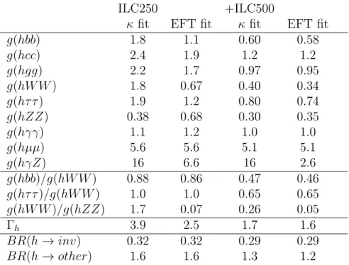
For this reason, it is well recognized that in the κformalism the measurement of the W W fusion cross section σ_ννh along with BR_{W W} (using the second half of (8)) is crucial for measurement of Γ_h and of all κ_A with A 6= Z. The expected precisions for Higgs boson couplings in the κ formalism are given in Table 1. We see that, at √

s = 250 GeV, κ_Z is determined very precisely, with accuracy of 0.38%, but most other κ_A are determined to no better than ∼ 2% (limited by σ_ννh and BR_ZZ measurements). An exception is κ_γ, which is helped significantly by the fact that the fit makes use of the expected measurement of BR_ZZ/BR_γγ at the HL-LHC.

4.3 Expected precisions for Higgs boson couplings in the EFT formalism In the EFT formalism, Higgs-Z interaction consists of two distinct Lorentz structures, shown in (4). As explained in the previous section, (9) is violated by the ζ_Z terms. Thus, the κ formalism is not model-independent, and it is not as general as the EFT formalism.

However, the EFT formalism allows Higgs boson couplings to be extracted via a much larger global fit. This fit includes not only the basic observables above but also additional observables of the reaction e⁺e⁻ → Zh, as well as observables of electroweak precision physics and e⁺e⁻ → W⁺W⁻. These latter measurements can

(17)

ILC250 +ILC500

κ fit EFT fit κ fit EFT fit

g(hbb) 1.8 1.1 0.60 0.58

g(hcc) 2.4 1.9 1.2 1.2

g(hgg) 2.2 1.7 0.97 0.95

g(hW W) 1.8 0.67 0.40 0.34

g(hτ τ) 1.9 1.2 0.80 0.74

g(hZZ) 0.38 0.68 0.30 0.35

g(hγγ) 1.1 1.2 1.0 1.0

g(hµµ) 5.6 5.6 5.1 5.1

g(hγZ) 16 6.6 16 2.6

g(hbb)/g(hW W) 0.88 0.86 0.47 0.46 g(hτ τ)/g(hW W) 1.0 1.0 0.65 0.65 g(hW W)/g(hZZ) 1.7 0.07 0.26 0.05

Γ_h 3.9 2.5 1.7 1.6

BR(h→inv) 0.32 0.32 0.29 0.29 BR(h→other) 1.6 1.6 1.3 1.2

Table 1: Projected relative errors for Higgs boson couplings and other Higgs observables, in %, for fits in theκ and EFT formalisms. The ILC250 columns assume a total integrated luminosity of 2 ab⁻¹at√

s= 250 GeV, shared by (−+,+−,−−,++) = (45%,45%,5%,5%) as described in Section 2. The ILC500 columns assume, in addition, a total integrated luminosity of 200 fb⁻¹ at√

s= 350 GeV, shared as (45%,45%,5%,5%), and a total integrated luminosity of 4 ab⁻¹ at√

s= 500 GeV, shared as (40%,40%,10%,10%). Three observables at the HL-LHC,BR_γγ/BR_ZZ,BR_γZ/BR_γγ andBR_µµ/BR_γγ, are included in all of the fits.

The effective couplingsg(hW W) andg(hZZ) are defined as proportional to the square root of the corresponding partial widths. The last two lines give 95% confidence upper limits on the exotic branching ratios. The detailed formulae used in the EFT fit, and the resulting covariance matrix, can be found in [15].

(18)

Precision of Higgs boson couplings [%]

0 2 4 6 8 10 12

g(hZZ)g(hWW) γ)

g(hγ g(hbb) g(hgg) τ) g(hτ g(hcc)

γZ) g(h

µ) g(hµ g(htt)

11% 14%

fit) κ (ATLAS: ATL-PHYS-PUB-2014-016 (2014), Model Dependent LHC 3000 fb-1

(Model Independent EFT fit) ILC 250 GeV, 2000 fb-1

⊕ LHC 3000 fb-1

(Model Independent EFT fit) 350 GeV, 200 fb-1

⊕ ILC 500 GeV, 4000 fb-1

⊕

ILC 250 GeV, 2000 fb-1

⊕ LHC 3000 fb-1

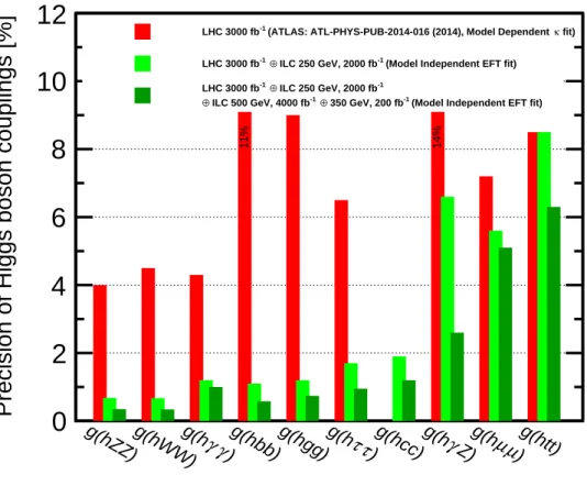
Figure 5: Illustration of the Higgs boson coupling uncertainties from fits in the EFT formalism, as presented in Table 1, and comparison of these projections to the results of model- dependent estimates for HL-LHC uncertainties presented by the ATLAS collaboration [23].

Earlier projections for HL-LHC are summarized in [28].

(19)

be included because the EFT Lagrangian is the complete Lagrangian and applies to all processes that occur ine⁺e⁻ annihilation. Though the number of free parameters is significantly increased, it turns out that each parameter can be well controlled experimentally. Then the EFT improves significantly the measurement of Higgs boson couplings. The detailed strategy is explained in Section 3 and in [15,19]. The results of Higgs boson coupling precisions based on the fitting program used in [15,19] are given in Table 1. These results are illustrated and compared to the projections of Higgs coupling uncertainties at HL-LHC from the ATLAS experiment [23] in Fig. 5.

While the EFT coefficients parametrize shifts in the Higgs couplings from massive new particles, the fit that we use also allows Higgs decays to new particles lighter than m_h/2, manifested both as invisible Higgs decays and as other modes of exotic decay.^§ The small difference with the numbers in [19] comes from the different luminosity sharing among (−+,+−,−−,++) assumed in the run plan presented in Section 2.

There are many interesting features in the Higgs boson coupling determination in the EFT formalism. It is worth emphasizing a few of them:

• A unique role is played by the inclusive Zh cross section, σ_Zh, enabled by the recoil mass technique. This remains the key element in the determination of the absolute normalization of all Higgs boson couplings. This freedom is mainly captured by the parameter c_H of the EFT formalism.

• The ratio of partial widths Γ(h → W W^∗)/Γ(h → ZZ^∗) is determined very precisely, to < 0.15%, mainly thanks to the constraints imposed on the EFT Lagrangian by SU(2)×U(1) gauge symmetry. In Table 1, we give values for effective couplings g(hW W), g(hZZ) defined to be proportional to the square roots of the partial widths. We see thatg(hW W) can be determined as precisely as g(hZZ) without relying on the σ_ννh measurement using the W W fusion process. This essentially solves the largest problem in measurement of Higgs boson couplings at √

s = 250 GeV. Note that once g(hW W) and g(hZZ) are determined, Γ_hand all other couplingsg(hAA) are determined straightforwardly using (8) and (10).

• In e⁺e⁻ →Zh, new observables making use of both cross section and angular information are included. The information in these observables is contained in two parameters a_Z, b_Z for each initial polarization state [29]. The parameter a_Z contains the η_Z term and is essentially identical for the polarizations e⁻_Le⁺_R and e⁻_Re⁺_L. The parameter b_Z contains ζ_Z orc_{W W} and also an effect of photon- Z mixing that is predicted by the EFT Lagrangian to depend on c_{W W} and related parameters. Estimates of the accuracy of the a_Z and b_Z measurements

§It is very conservative at an e⁺e⁻ collider to allow that as many as 1% of Higgs decays will remain unrecognized as distinct processes. However, we do allow this for the purpose of this fit.

(20)

Figure 6: Contour plots foraZ versusbZ from [29]: for√

s= 250 GeV with 250 fb⁻¹ (left);

for√

s= 500 GeV with 500 fb⁻¹ (right).

Z

h Z h Z

A h

Figure 7: Feynman diagrams contributing to the amplitudes fore⁺e⁻→Zh.

for individual polarization states, based on full detector simulation described in [29], are given in the Appendix of [19]. It is found that accuracies of the a_Z and b_Z determinations at 250 GeV are rather limited compared to that at 500 GeV; see Fig. 6. Luckily, there are other powerful means to help constrain c_{W W}.

• The photon-Z mixing effect that contributes to b_Z leads an additional diagram fore⁺e⁻ →Zhwith ans-channel photon instead of aZ. This diagram is shown in Fig. 7 along with a third diagram that arises from dimension-6 operator vertices. The interference between the first two diagrams is constructive for e⁻_Le⁺_R and destructive for e⁻_Re⁺_L. Since the mixing effect depends strongly on c_{W W}, this EFT coefficient can be constrained very well using measurement of the polarization asymmetry in σ_Zh. Note that this polarization asymmetry in σZH can be determined from usingσZh·BRmeasurements (which can be done with hadronic decay modes of the Z) as well as from inclusive cross section

(21)

measurements (which are dominated by leptonic decays of the Z). This allows more of the total data set to be used to constrain c_{W W}. The overall effect of beam polarizations on the determination of Higgs boson couplings can be found in Table 4 of [19].

• The decays h → γγ and h → Zγ are loop-induced in the SM, but receive corrections at the tree level from dimension-6 operators. Thus, Γγγ and ΓZγ

are very sensitive to the operator coefficients c_{W W}, c_{W B} and c_BB, the same set of operators that determine ζ_A, ζ_AZ, ζ_Z and ζ_W. The measurements of BRZZ/BRγγ and BRγZ/BRγγ from the HL-LHC turn out to be very helpful, providing tight constraints on two linear combinations of c_{W W}, c_{W B} and c_BB, even though the projected accuracy for the Zγ decay is only 31% [23]. It will be interesting to study whether any observable at ILC can measure the hZγ coupling directly to still better accuracy.

• The Triple Gauge Couplings (TGCs) measured in e⁺e⁻ →W⁺W⁻ play a very important role in fixing three of the 17 relevant EFT coefficients. So it is important that ILC will dramatically improve the measurement of TGCs over what has been accomplished at LEP2 and LHC. We will discuss this measurement in Section 8 below.

• The rightmost diagram in Figure 7 is induced by contact interactions from dimension-6 operator coefficients that correct the Z-lepton vertices measured from precision electroweak observables. These parameters appear in σ_Zh with very large coefficients, of order 2s/m²_Z ∼ 15 (60) at √

s = 250 (500) GeV. It turns out that the constraints on these coefficients is improved over that from the current precision electroweak measurements by the comparison of Higgs cross sections at 250 and 500 GeV.^¶Alternatively, the EFT fit would be assisted by improvement of precision electroweak measurements, either by direct e⁺e⁻ running at theZ pole or by measurements of the polarization asymmetry of the radiative return process e⁺e⁻ → Zγ. This is another topic that needs further investigation.

4.4 Measurement of the Higgs boson mass and CP

The uncertainty in the Higgs boson mass (δm_h) is a source of systematic error for predictions of Higgs boson couplings. In most cases, δmh ∼ 0.2% would be already sufficient, but this is not true for h → ZZ^∗ or h → W W^∗. It has been pointed out in [30] that

δW = 6.9·δmh, δZ = 7.7·δmh, (11)

¶The fit described here uses only the current uncertainties in precision electroweak measurements, except for an improvement in the uncertainty in ΓW to 0.1% expected from ILC measurements of final states ine⁺e⁻→W⁺W⁻.

(22)

whereδ_W andδ_Z are the relative errors forg(hW W) andg(hZZ) respectively. At the 250 GeV ILC, the Higgs boson mass can be measured very precisely, with an accuracy of 14 MeV using the leptonic recoil channel as shown in Fig. 4 (left). This results in systematic errors for δ_W and δ_Z of 0.1%. The study of the new beam parameters discussed in Section 2, which would increase the beamstrahlung effect significantly, should pay attention to this issue.

At the 250 GeV ILC, Higgs CP properties can be probed via the hτ τ coupling,

∆Lhτ τ =−κ_τy_τ

√2 hτ⁺(cosφ+isinφγ5)τ⁻ (12) and thehV V coupling

∆L_hZZ = 1 2

˜b

vhZ_µνZ˜^µν. (13) The CP phase φ in (12) can be measured with an accuracy of 3.8^◦ [31], and ˜b in (13) can be measured with an accuracy of 0.5% [29]. The observation of even a small admixture of CP-odd coupling for the Higgs boson would indicate physics beyond the Standard Model, and might give a clue to the CP violation required in models of electroweak baryogenesis.

5 Comparison of the ILC capabilities for the Higgs boson to the predictions of new physics models

Now that we have presented the expectations for the accuracy of ILC measurements of the Higgs boson couplings, it is important to ask whether these expectations are strong enough to search for new physics beyond the reach of direct searches at the LHC. We will discuss that point in this section. First, we will survey models of new physics that affect the Higgs boson, review the diversity of models under consid- eration, and present the effects on the Higgs couplings predicted in the various types of models. Then we will present a representative sample of specific model points that demonstrate the power of the ILC measurements.

5.1 Models of electroweak symmetry breaking and the Higgs field

Our present understanding of the breaking of theSU(2)×U(1) gauge symmetry of the SM is crude and unsatisfactory. This point is, suprisingly, more easily grasped by condensed matter physicists than by particle physicists. Condensed matter physicists are familiar with the history of superconductivity, for which the basic understanding developed in two stages. In 1950, Landau and Ginzburg wrote a phenomenologi- cal theory of superconductivity that was, in fact, the model for the theory of the

(23)

Higgs field [32]. This model was successful and even predictive of many aspects of superconductivity, but, in this model, the basic fact of the phase transition to superconductivity was put in by hand. Only later, in 1957, did Bardeen, Cooper, and Schrieffer (BCS) create a fundamental theory of superconductivity based on pairing of electrons in a metal [33]. The BCS theory was not only a conceptual improvement but also predicted many new features of superconductivity that were beyond the reach of the Landau-Ginzburg description. In particle physics, we are now at the Landau-Ginzburg stage [34]. The difference from the condensed matter situation is that the interactions that drive electroweak symmetry breaking and lead to the phase transition must be new interactions, outside the SM, that have not yet been discovered. Thus, the exploration of the Higgs field offers the opportunity to discover genuinely new interactions of nature.

Many features of the SM argue that it cannot be a fundamental solution for electroweak symmetry breaking. For example, there are good reasons to believe that a scalar boson cannot be light (compared to Planck scale, for example) and give mass to all other particles in the SM without aid from other—as yet undiscovered—particles and interactions. These additional particles necessarily interact with the Higgs boson and can change the expectations for Higgs couplings to SM states.

Theories of physics beyond the SM are constructed to solve one or more outstand- ing problems that the SM does not address. They might attempt to explain the low mass of the Higgs boson without large fine-tunings as discussed above; they might posit dark matter candidates; they might explain the baryon asymmetry of the universe; they might unify the SM forces. In this space of theories there are many that can produce experimentally accessible non-SM signals to be discovered in the near term — some through direct searches of particles at the LHC’s high-energy frontier, and others through a myriad of other experiments currently running or planned for the near future. Among these probes, though, precision measurement of the Higgs couplings is one of the most powerful. The reasons for this are two-fold. First, the Higgs sector is where we expect the most new interactions in many beyond the SM theories. Second, measurements in the Higgs sector have great room for improvement over current precision levels that can reveal new physics effects for beyond the SM theories that no other experiments could access.

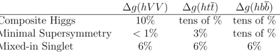
Models that address the problems just listed can be constructed using many different approaches. A survey of these approaches, and estimates of the maximum possible effect on the Higgs boson couplings, was given in [35]. Table 2 lists three important classes of models and the corresponding estimates for maximal deviations in different couplings of the Higgs boson.

One class of models builds on the analogy with superconductivity. The order parameter for the Landau-Ginzburg potential of superconductivity turned out to be a composite state of electrons (Cooper pairs). It has been suggested that the Higgs

(24)

∆g(hV V) ∆g(htt) ∆g(hbb) Composite Higgs 10% tens of % tens of % Minimal Supersymmetry <1% 3% tens of %

Mixed-in Singlet 6% 6% 6%

Table 2: Estimated maximum deviations of Higgs couplings to various SM states allowed by three different scenarios of physics beyond the SM. The assumption is that no new physics associated with electroweak symmetry breaking is found at the HL-LHC (3 ab⁻¹ at

√s= 14 TeV), and thus Higgs coupling measurements are the only potential signal for new physics. Adapted from [35].

boson state is also composite. If this is true, it has the potential to explain the large hierarchy between the Higgs mass and the Planck scale. A collection of some of the simplest approaches along this line leads to potentially large deviations of Higgs boson couplings to SM states compared to the expected measurement accuracies from the ILC.

A different class of models makes use of supersymmetry. Supersymmetry posits a symmetry between bosons and fermions that not only could explain the Higgs boson mass with respect to the Planck mass, but it could also be the source of dark matter, and it could be the key ingredient that enables the unification of forces at the high scale [36]. The symmetry requirements of supersymmetry require the introduction of two Higgs bosons – one that gives mass to up-type fermions and one that gives mass to down-type fermions. The two Higgs doublets mix and leave one CP-even eigenstate light, which is identified with the 125 GeV Higgs boson (h). It is straightforward to derive that this light boson h has couplings identical to those of the SM Higgs boson except for small deviations that are induced by mixings with the extra Higgs states and loop corrections involving the superpartners and the heavy Higgs bosons.

These deviations of couplings can be well above 10% in the case of Higgs coupling to b quarks, even if no superpartner is ever found at the LHC in all its planned upgrade phases [35]. This is illustrated nicely by Fig. 8, where the authors scanned over hundreds of thousands of MSSM supersymmetric points [37]. They showed that many sets of parameters in the MSSM can never be found at the LHC but would be easily discernible through precision measurements at the ILC.

A third class of models postulates additional scalar fields. After all, there are many fermions, and there are many vector bosons. Multiple scalars are already required within supersymmetry, where in addition to scalar superpartners we stated that two Higgs bosons are required. But there are many more ideas of beyond the SM physics that incorporate several scalar bosons but do not cause ill effects elsewhere, by, for example, inducing too large flavor changing neutral currents. These multi-Higgs doublet models are classified as type I (in which one Higgs gives mass to fermions, and the other does not), type II (in which one Higgs gives mass to up fermions only

(25)

0.5 1.0 1.5 2.0 2.5 3.0 3.5

r _bb

10

^-1

10

⁰

10

¹

10

²

10

³

10

⁴

Number of models

All models

After current searches After 14 TeV 300 fb

⁻¹

After 14 TeV 3000 fb

⁻¹

Figure 8: Histograms of the ratio r_bb = Γ(h → bb)/Γ(h → bb)_SM within a scan of the approximately 250,000 supersymmetry parameter sets after various stages of the LHC, assuming the LHC does not find direct evidence for supersymmetry. The purple histogram shows parameter points that would not be discovered at future upgrades of the LHC (14 TeV and 3 ab⁻¹ integrated luminosity). From [37].

(26)

Model bb cc gg W W τ τ ZZ γγ µµ

1 MSSM [37] +4.8 -0.8 - 0.8 -0.2 +0.4 -0.5 +0.1 +0.3

2 Type II 2HD [38] +10.1 -0.2 -0.2 0.0 +9.8 0.0 +0.1 +9.8

3 Type X 2HD [38] -0.2 -0.2 -0.2 0.0 +7.8 0.0 0.0 +7.8

4 Type Y 2HD [38] +10.1 -0.2 -0.2 0.0 -0.2 0.0 0.1 -0.2

5 Composite Higgs [39] -6.4 -6.4 -6.4 -2.1 -6.4 -2.1 -2.1 -6.4 6 Little Higgs w. T-parity [40] 0.0 0.0 -6.1 -2.5 0.0 -2.5 -1.5 0.0 7 Little Higgs w. T-parity [41] -7.8 -4.6 -3.5 -1.5 -7.8 -1.5 -1.0 -7.8 8 Higgs-Radion [42] -1.5 - 1.5 +10. -1.5 -1.5 -1.5 -1.0 -1.5 9 Higgs Singlet [43] -3.5 -3.5 -3.5 -3.5 -3.5 -3.5 -3.5 -3.5 Table 3: Percent deviations from SM for Higgs boson couplings to SM states in various new physics models. These model points are unlikely to be discoverable at 14 TeV LHC through new particle searches even after the high luminosity era (3 ab⁻¹ of integrated luminosity).

From [19].

and one to down fermions only), and type X and Y models (with more complicated discrete symmetries that protect flavor observables) [38].

5.2 Comparisons of models to the ILC potential

All of these ideas lead to models with deviations from the SM expectations of the couplings of the 125 GeV Higgs boson to SM states. Table 3collects a set of models of new physics based on the ideas described in the previous section and on several additional ideas of interest to theorists. For each model, we chose a representative parameter point for which the predicted new particles would be beyond the reach of the 14 TeV LHC with the full projected data set. The deviations of Higgs couplings from the SM expectations at these representative model points are listed in the Table.

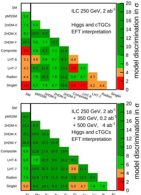
(For details, see [19] as well as the papers cited in Table3.) These examples illustrate diverse possibilities for models with significant deviations of the Higgs couplings from the SM expectation that would be allowed even if the LHC and other experiments are not able to discover the corresponding new physics beyond the SM. We should make clear that the quantitative statements to follow refer to these particular models at the specific parameter points shown in the Table. Figure 9 shows graphically the ability of ILC measurements to distinguish the Higgs boson couplings in the models in the Table from the SM expectations and from the expectations of other models. Each square shows relative goodness of fit for the two models in units ofσ. The top figure is based on the covariance matrix from the 250 GeV stage of the ILC, corresponding to the second column of Table1. The bottom figure reflects the full ILC program with 500 GeV running, corresponding to the fourth column of Table 1. It is noteworthy that, once it is known that the Higgs boson couplings deviate significantly from the

(27)

σ model discrimination in

0 2 4 6 8 10 12 14 16 18 20

SM pMSSM2HDM-II2HDM-X2HDM-YCompositeLHT-6 LHT-7 RadionSinglet Singlet

Radion LHT-7 LHT-6 Composite 2HDM-Y 2HDM-X 2HDM-II pMSSM SM

2.4 5.7 7.9 6.7 10.5 2.5 2.6 4.2 4.4 4.4 7.8 10.3 7.8 12.2 5.0 6.7 4.7 4.1 8.3 11.5 7.9 13.1 2.0 6.3 3.1 4.6 5.8 6.7 9.3 4.4 2.8 6.8 9.7 7.1 11.6 10.1 5.6 7.7 15.1

6.1 10.0 9.2 7.4 5.4 5.0

ILC 250 GeV, 2 ab-1

Higgs and cTGCs EFT interpretation

σ model discrimination in

0 2 4 6 8 10 12 14 16 18 20

SM pMSSM2HDM-II2HDM-X2HDM-YCompositeLHT-6 LHT-7 RadionSinglet Singlet

Radion LHT-7 LHT-6 Composite 2HDM-Y 2HDM-X 2HDM-II pMSSM SM

5.0 9.4 14.1 9.3 17.0 5.0 4.7 7.8 7.8 7.6 12.9 17.9 11.3 20.0 8.9 11.5 8.5 7.6 14.6 20.5 11.5 22.1 3.6 11.4 5.8 7.0 10.3 9.6 14.2 8.1 5.5 11.8 17.4 10.0 19.5 16.0 8.6 10.2 21.9

8.1 14.0 15.1 13.2 8.3

8.0 -1

+ 350 GeV, 0.2 ab + 500 GeV, 4 ab-1

ILC 250 GeV, 2 ab-1

Higgs and cTGCs EFT interpretation

Figure 9: Graphical representation of the χ² separation of the Standard Model and the models 1–9 described in the text: (a) with 2 ab⁻¹ of data at the ILC at 250 GeV; (b) with 2 ab⁻¹ of data at the ILC at 250 GeV plus 4 ab⁻¹ of data at the ILC at 500 GeV.

Comparisons in orange have above 3 σ separation; comparison in green have above 5 σ separation; comparisons in dark green have above 8 σ separation. From [19], with slight

(28)

SM predictions, the pattern of the deviations is characteristic for each model and distinguishable from the patterns predicted by other models in the set.

The evidence for significant deviations in the Higgs boson couplings would demonstrate that there is new physics beyond the SM that affects the Higgs field. The observation of the pattern of deviations would give us information on the properties of this new physics and point the way to further model-building and experimental exploration. This is a route to a deeper understanding of nature that the ILC offers us.

6 Invisible and exotic Higgs decays

In addition to the expected decays of the Higgs boson whose analysis was discussed in the previous two sections, the Higgs boson could also have additional decay modes that are not predicted by the SM. The ILC at 250 GeV will accumulate a data set containing half a million Higgs bosons tagged by recoilingZ bosons. This will provide an ideal environment to search for any possible final state of Higgs decay.

Exotic decays of the Higgs boson are expected in many theoretical models. An attractive way to model the dark matter of the universe is to assume the existence of a “hidden sector” consisting of one or more fields with no SM gauge charges. Since particles of a hidden sector do not couple through gauge forces, their interactions with SM particles are highly model-dependent and can be very feeble. Such particles can be consistent with all existing experimental constraints even if their masses are well below the weak scale. If some of the hidden-sector particles are stable, these could make up the observed dark matter. For example, in the “Strongly-Interacting Massive Particle” (SIMP) scenario [44,45], dark matter consists of mesons produced by confinement of a QCD-like gauge group in the dark sector. A light hidden sector also appears in well-motivated theoretical models of electroweak symmetry breaking such as the “Twin Higgs” model [46]. Hidden-sector particles have also been in- voked as an explanation of the apparent discrepancy between the experimental and theoretical values of the anomalous magnetic moment of the muon, and a number of other experimental anomalies. In light of this, there is strong interest in experimental searches for these particles, and a number of approaches are currently being pursued or studied [47,48].

To connect the hidden-sector particles to initial states with Standard Model particles, it is necessary to add a term to the Lagrangian that connects these sectors.

There are precisely three dimension-4 operators that can make this connection:

B_µνFˆ^µν , |ϕ|²|S|ˆ² , L^†·ϕN ,ˆ (14) where Bµν is the U(1) field strength, ϕ is the Higgs doublet, and L is the lepton