Variational Inequality Approaches to Generalized Nash Equilibrium Problems

Variational Inequality Approaches to Generalized Nash Equilibrium Problems

Guidance

Professor Masao FUKUSHIMA

Koichi NABETANI

2006 Graduate Course in

Department of Applied Mathematics and Physics Graduate School of Informatics

Kyoto University

KYOTO UNIVERS ITY

FO

U^KYOTON DED 1^JAPAN897

February 2008

Abstract

We consider the generalized Nash equilibrium problem (GNEP), in which each player’s strategy

set may depend on the rivals’ strategies. The GNEP can be formulated as a quasi-variational

inequality (QVI). However, unlike the standard variational inequality (VI), there are only a few

methods available for solving a QVI efficiently. A practical approach to find a GNE is to solve

a related VI rather than solving the corresponding QVI directly, and it has been receiving much

attention recently. From the viewpoint of game theory, it is important to find GNEs as many

as possible, or all of them if possible. We propose the price-directed and the resource-directed

parametrization methods that construct parametrized families of VIs related to the GNEP. We

then show that those VIs yield all GNEs under suitable conditions. Moreover, by means of some

numerical examples, we show that GNEs obtained by the proposed VI approaches are widely

distributed in the GNEP solution set.

Contents

1 Introduction 1

2 Problem Formulation and Assumptions 2

3 Parameterized VI Approaches to GNE with Shared Constraints 4 3.1 Price-Directed Parametrization . . . . 5 3.2 Resource-Directed Parametrization . . . . 8 3.3 Relation between some GNE concepts and VI approaches . . . . 10

4 Numerical Experiments 13

4.1 Examples . . . . 13 4.2 Numerical Results . . . . 15

5 Concluding Remarks 21

1 Introduction

The generalized Nash equilibrium problem (GNEP) is a generalization of the standard Nash equi- librium problem (NEP), in which each player’s strategy set may depend on the rivals’ strategies [1, 23, 8]. Recently, the GNEP has attracted much attention [5, 14] because there are many interesting applications in the fields of economics, mathematics and engineering. For example, Robinson [20, 21] discussed a two-sided game model of combat as an application of GNEP. Wei and Smeers [26] and Hobbs [11] formulated oligopolistic electricity models as GNEPs.

It is well known that NEP where each player solves a convex programming problem can be formulated as a finite-dimensional variational inequality (VI) [9, 6]. The VI has a long history and the state-of-the-art and various computational methods are presented in the recent monograph [6]. On the other hand, GNEP can be formulated as a quasi-variational inequality (QVI) [8, 19].

However, unlike the VI, there are only a few methods available for computing a generalized Nash equilibrium (GNE) or solving a QVI efficiently [17, 19, 18]. A practical approach to GNEP is to find a GNE via a VI rather than solving a QVI directly [8, 26, 18, 19, 3, 4] and it has received much attention recently.

Pang and Fukushima [19] propose a penalty method for GNEP, which solves a sequence of penalized NEPs, and establish its convergence under some assumptions. Pang [18] formulates GNEP as a partitioned VI via the equivalent Karush-Kuhn-Tucker (KKT) system and proposes to apply the Josephy-Newton method that solves a linearized VI at each iteration. Local superlinear convergence is established under convexity and regularity assumptions.

Wei and Smeers [26] formulate an oligopolistic electricity model as a GNEP with “shared constraints”, which means the constraint functions that depend on rivals’ strategies are identical among all players. They present a VI formulation such that its solution is GNE, and establish the uniqueness of GNE under some restrictive assumptions. Facchinei et al. [3] also consider a GNEP with shared constraints and propose to apply Newton-type methods to solve its VI formulation.

This approach seems to be promising because we can find a GNE by solving a single VI. However, the obtained GNE is a particular equilibrium such that the multipliers of the shared constraints are identical [3, 4]. In general, GNEP has multiple, or even infinitely many, solutions [8]. In practical situations, the players usually have different objective functions, and the multipliers of the shared constraints need not be identical. Therefore, the VI formulation considered in [26, 3, 4]

may fail to identify some important GNEP solutions.

Another approach for GNEP is the algorithms [24, 13, 10] based on the Nikaido–Isoda function [16]. Uryasev and Krawczyk [24, 13] develop the relaxation method and establish the global convergence of the algorithm under some assumptions, which are, however, rather restrictive. In a recent paper, von Heusinger and Kanzow [10] consider the regularization of the Nikaido–Isoda function and reformulate a GNEP with shared constraints as a smooth optimization problem.

However, it is shown that these methods also find only a part of GNEP solutions in general.

From the practical viewpoint of game theory, it is important to find as many GNEs as possible, or all of them if possible [25]. To the best of our knowledge, little attempt has been made to develop a method to achieve this. The goal of the present paper is to construct, for GNEP with shared constraints, a parametrized family of VIs whose solutions include all GNEs. This extends the VI approaches studied in [26, 3, 4] and show that all GNEP solutions are contained in the solution sets of those VIs. Moreover, we clarify the conditions that guarantee a solution of those VIs to be a GNE.

The paper is organized as follows. In the next section, we recall some definitions and basic

concepts. In Section 3, we present the parametrized family of VIs and show that those VIs yield

all GNEP solutions. We also show that the parameters involved in VIs can be restricted to a

bounded set. In Section 4, we present some numerical results with the proposed approach. Finally, Section 5 concludes the paper.

We use the following notations throughout the paper. For a set X, P (X) denotes the set of all subsets of X. For a nonempty closed convex set X ⊂ ⁿ , N _X (x) = { d ∈ ⁿ | d ^T (y − x) ≤ 0 ∀ y ∈ X } denotes the normal cone to X at x ∈ X. For a function f : ⁿ × ^m → , f (x, · ) : ^m → denotes the function with x being fixed. We denote the nonnegative and positive orthants in ⁿ by ⁿ ₊ and ⁿ ₊₊ , respectively, that is,

ⁿ ₊ := { x ∈ ⁿ | x ≥ 0 } and ⁿ ₊₊ := { x ∈ ⁿ | x > 0 } .

For vectors x, y ∈ ⁿ , x, y denotes the inner product defined by x, y := x ^T y and x ⊥ y means x, y = 0. For a vector x, x denotes the Euclidean norm defined by x :=

x, x . A mapping F : ⁿ → ⁿ is said to be monotone on a nonempty closed convex set X ⊂ ⁿ if

F (x) − F (y), x − y ≥ 0 ∀ x, y ∈ X,

strictly monotone on X if the above inequality is strict whenever x = y, and strongly monotone on X if zero on the right-hand side of the above inequality is replaced by α x − y ² for some constant α > 0.

2 Problem Formulation and Assumptions

The generalized Nash game with N players is to find a profile of strategies such that each player’s strategy is an optimal response to the rival players’ strategies, where each player’s strategy set may depend on the rival players’ strategies. For ν = 1, . . . , N, let x _ν ∈ ⁿ

be a player ν’s strategy, where n _ν is a positive integer. The vector formed by all these strategies is denoted x := (x _ν ) ^N _ν=1 ∈ ⁿ , where n := _N

ν=1 n _ν , and the vector formed by all the players’ strategies except those of player ν is denoted x

:= (x _ν

) ^N _ν

_{=1, ν}

∈ ⁿ

, where n

:= n − n _ν . For ν = 1, . . . , N, let K _ν be a given point-to-set mapping from ⁿ

to ⁿ

. Thus, for each fixed x

, K _ν (x

) is a subset of ⁿ

, which is the strategy set of player ν with the other players’ strategies given by x

.

Each player ν = 1, . . . , N , taking the other players’ strategies x

as exogenous variables, solves the minimization problem:

P _ν (x

) : minimize θ _ν (x _ν , x

)

subject to x _ν ∈ K _ν (x

), (1)

where θ _ν : ⁿ → is a given cost function of player ν. A vector x = (x _ν ) ^N _ν=1 is said to be feasible to GNEP if x _ν ∈ K _ν (x

) for each ν = 1, . . . , N.

The GNEP is to find a vector x

= (x

_ν ) ^N _ν=1 ∈ ⁿ such that

x

_ν is an optimal solution of P _ν (x

) for all ν = 1, . . . , N. (2) A vector x

satisfying (2) is called a generalized Nash equilibrium (GNE). The set of GNEs is denoted by SOL

.

In many practical applications, the strategy set K _ν (x

) of player ν is represented by finitely many inequality constraints. In particular, we assume that the feasible strategy set K _ν (x

) of player ν has the form

K _ν (x

) = { x _ν ∈ X _ν | g _ν (x _ν , x

) ≤ 0 } , (3)

where g _ν = (g _ν,i ) ^m _i=1

: ⁿ → ^m

and X _ν ⊂ ⁿ

, with m _ν a nonnegative integer. Thus, player ν’s strategy is constrained in two ways; joint constraints that depend also on the other players’

strategies, i.e., g _ν (x) ≤ 0, and individual constraints that depend only on player ν ’s strategy, i.e., x _ν ∈ X _ν . In what follows, we let

X

:=

N ν

=1 ν

X _ν

.

We distinguish these two types of constraints since our parametrization will involve only the joint constraints. Throughout this paper, we make the following blanket assumption on the smoothness and convexity of functions involved in the GNEP.

Assumption A. For ν = 1, . . . , N , the set X _ν is nonempty, closed, convex, and, for each fixed x

∈ X

, the functions θ _ν ( · , x

) and g _ν,i ( · , x

), i = 1, . . . , m _ν , are differentiable and convex.

By Assumption A, problem (1) is a differentiable convex programming problem. Thus a nec- essary and sufficient condition for x

_ν ∈ K _ν (x

) to be optimal for (1) is that the inequalities

∇ _x

θ _ν (x

_ν , x

), x _ν − x

_ν ≥ 0 ∀ x _ν ∈ K _ν (x

) hold. Thus, by defining

F (x) := ( ∇ _x

θ _ν (x _ν , x

)) ^N _ν=1 , (4) K(x) :=

N ν=1

K _ν (x

), it follows that x

is a GNE if and only if x

∈ K(x

) and

F(x

), x − x

≥ 0 ∀ x ∈ K(x

).

The latter problem is a QVI, which we denote by QVI (F, K).

Suppose that x

is a solution of GNEP. Then, for each ν = 1, . . . , N , x

_ν is an optimal solution of the convex programming problem:

P _ν (x

) : minimize θ _ν (x _ν , x

)

subject to g _ν (x _ν , x

) ≤ 0, x _ν ∈ X _ν .

Under a suitable CQ at x

(see, e.g., [2, Section 5.4], [22]), there exists for each ν = 1, . . . , N a vector λ

_ν ∈ ^m

satisfying the Karush-Kuhn-Tucker (KKT) condition:

0 ∈ ∇ _x

L _ν (x _ν , x

, λ _ν ) + N _X

(x _ν ),

0 ≤ λ _ν ⊥ g _ν (x _ν , x

) ≤ 0, x _ν ∈ X _ν , (5) where the Lagrangian function L _ν is defined by

L _ν (x, λ _ν ) := θ _ν (x) + g _ν (x), λ _ν .

The vector λ

= (λ

_ν ) ^N _ν=1 is called a Lagrange multiplier vector. Under Assumption A, if (x

, λ

) satisfies (5), then x

is a GNE. A well-known CQ at x is the Mangasarian-Fromovitz CQ (MFCQ) [22, page 198]:

0 ∈ ∇ _x

g _ν (x)λ _ν + N _X

(x _ν ), 0 ≤ λ _ν ⊥ g _ν (x) ≤ 0, x _ν ∈ X _ν

= ⇒ λ _ν = 0, ν = 1, . . . , N,

where

∇ _x

g _ν (x) :=

∇ x

g _ν,1 (x) · · · ∇ x

g _ν,m

(x) .

Another useful CQ at x is the Linear Independence CQ (LICQ):

0 ∈ ∇ _x

g _ν (x)λ _ν + N _X

(x _ν ) + (−N _X

(x _ν )), λ _ν ⊥ g _ν (x) ≤ 0, x _ν ∈ X _ν

= ⇒ λ _ν = 0, ν = 1, . . . , N. (6) This CQ implies uniqueness of the multiplier vector λ

for each x

.

3 Parameterized VI Approaches to GNE with Shared Constraints

In this section, we consider the case of “shared constraints”, that is, all players share common constraints that depend on all the players’ strategies. Specifically, we make the following blanket assumption.

Assumption B. For some m ¯ and g = (g _i ) ^m _i=1 ^¯ : ⁿ → ^{m ¯} , we have m ₁ = · · · = m _N = ¯ m and g ¹ = · · · = g ^N = g. Moreover, g _i : ⁿ → is differentiable and convex for all i = 1, . . . , m.

Then, (x

, λ

) satisfies the KKT condition (5) if and only if (x

, λ

) satisfies 0 ∈ ∇ _x

θ _ν (x) + ∇ _x

g(x)λ _ν + N _X

(x _ν ), ν = 1, . . . , N,

0 ≤ λ _ν ⊥ g(x) ≤ 0, x _ν ∈ X _ν , ν = 1, . . . , N.

(7) Note from the complementarity condition that g _i (x) < 0 implies that λ _ν,i = 0 for all ν = 1, . . . , N and λ _ν,i > 0 for some ν implies that g _i (x) = 0.

The VI approach to finding a GNE [26, 3, 4] is to define

X := { x ∈ X ₁ × · · · × X _N | g(x) ≤ 0 } ,

which is a closed convex (possibly empty) set, and solve the following VI (F, X):

Find x

∈ X such that F (x

), x − x

≥ 0 ∀x ∈ X,

where F : ⁿ → ⁿ is defined by (4). The solution set of VI (F, X) is denoted by SOL (F, X) ¹ . A vector x

belongs to SOL (F, X) if and only if it is an optimal solution of the convex programming problem:

minimize F (x

), x

subject to x ∈ X, (8)

whose KKT condition is a special case of (7) with λ ₁ = · · · = λ _N . Specifically, the following result is known [3, Theorem 3.6] (also see [26, Theorem 2] and [4, Theorem 2.1]).

Theorem 3.1. Every x

∈ SOL (F, X) is a GNE. Furthermore, if x

together with some Lagrange multiplier vector satisfies the KKT condition for (8), then x

and some λ

= (λ

_ν ) ^N _ν=1 with λ

₁ =

· · · = λ

_N satisfy (7).

1

A solution of VI (F, X) is called a variational equilibrium in [5] and is shown to be a particular instance of a

normalized equilibrium introduced by Rosen [23]. In Section 3.3, we will show the relation between normalized

equilibrium and the solutions of VI formulations.

In many practical situations, since the players have different objective functions as well as their own constraints, the multipliers of the shared constraints in GNEP may not be identical.

Therefore, in general, there would be many GNEs that are not normalized equilibria. This is illustrated in the following example.

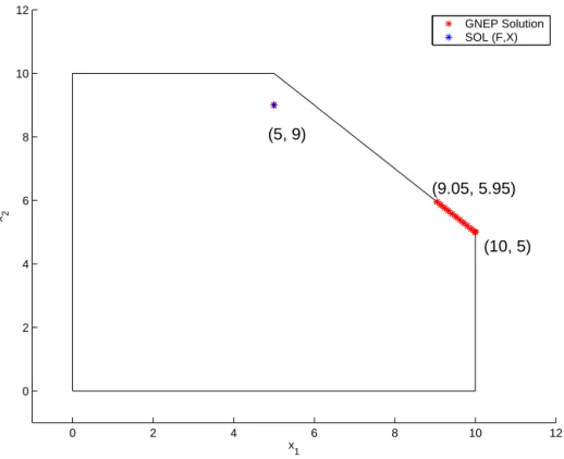
Example 1. Consider the two-person game, where the problems of player 1 and player 2 are defined by

P ₁ (x ₂ ) : minimize x ² ₁ − x ₁ x ₂ − x ₁ subject to x ₁ ≥ 0

x ₁ + x ₂ ≤ 1, and

P ₂ (x ₁ ) : minimize x ² ₂ − ¹ ₂ x ₁ x ₂ − 2x ₂ subject to x ₂ ≥ 0

x ₁ + x ₂ ≤ 1, respectively. The set of GNEs consists of infinitely many vectors

x ₁ x ₂

= t

1 − t

, 0 ≤ t ≤ ² ₃ .

On the other hand, the corresponding F : ² → ² and X ⊆ ² are given by F (x) = 2x ₁ − x ₂ − 1

− ¹ ₂ x ₁ + 2x ₂ − 2

, X = {x ∈ ² ₊ | x ₁ + x ₂ ≤ 1}, and the solution of VI (F, X) is uniquely given by x = ₄

11 , ₁₁ ⁷ _T .

In this example, the mapping F is strongly monotone and hence SOL (F, X) is a singleton [6], but there are infinitely many GNEs. Uniqueness of GNE requires restrictive assumptions [8, 26]

which cannot be expected to hold in most applications. In general, the above VI approach can find only a part of the GNEs.

3.1 Price-Directed Parametrization

Now, we construct a family of VIs that contains VI (F, X) as a particular instance. Let Δ = (Δ _ν ) ^N _ν=1 ∈ ^m ₊ with m = N m ¯ and Δ _ν ∈ ^m ₊ ^¯ , ν = 1, . . . , N, be a vector of parameters. Define the function F ^Δ : ⁿ → ⁿ by

F ^Δ (x) := ( ∇ x

θ _ν (x) + ∇ x

g(x)Δ _ν ) ^N _ν=1 . (9) Note that VI (F ^Δ , X) reduces to VI (F, X) if the parameter Δ is set to be zero. The follow- ing proposition shows that, under appropriate assumptions, the monotonicity of F implies the monotonicity of F ^Δ for any Δ ∈ ^m ₊ .

Proposition 3.1. Assume that F is monotone (strictly monotone, strongly monotone) on X.

Assume further that the shared constraint function g is separable, that is, g(x) can be written as g(x) =

N ν=1

ˆ

g _ν (x _ν ), (10)

where ˆ g _ν = (ˆ g _ν,i ) ^m _i=1 ^¯ : ⁿ

→ ^{m ¯} , ν = 1, . . . , N, are differentiable convex functions. Then, for

any Δ ∈ ^m ₊ , F ^Δ is also monotone (strictly monotone, strongly monotone) on X.

Proof. Since g is separable, we have

F ^Δ (x) = F (x) + ( ∇ g ˆ _ν (x _ν )Δ _ν ) ^N _ν=1 .

For each ν = 1, . . . , N and i = 1, . . . , m, ¯ ∇ g ˆ _ν,i is monotone on X _ν since ˆ g _ν,i is a differentiable convex function. Therefore F ^Δ is monotone (strictly monotone, strongly monotone) on X for any Δ ∈ ^m ₊ .

Under the assumptions of this proposition, we can apply, for example, Newton-type or projection- type methods to solve VI (F ^Δ , X). A sufficient condition for F to be strictly monotone in the setting of spatial oligopolistic electricity models is given in [26, Theorems 5 and 6].

We now investigate the relationship between VI (F ^Δ , X) and GNEP. The KKT condition for VI (F ^Δ , X) can be written as

0 ∈ ( ∇ _x

θ _ν (x) + ∇ _x

g(x)Δ _ν ) + ∇ _x

g(x)π + N _X

(x _ν ), ν = 1, . . . , N, 0 ≤ π ⊥ g(x) ≤ 0, x _ν ∈ X _ν , ν = 1, . . . , N.

(11) For each GNE x, let

M (x) := { λ ∈ ^m | (x, λ) satisfies the KKT condition (7) } . By comparing this KKT condition (11) with (7), we have the following result.

Theorem 3.2. For any GNE x

, if λ

∈ M (x

), then x

∈ SOL (F ^λ

, X).

Proof. Fix any GNE x

, and assume that λ

∈ M (x

). Then (x

, λ

) satisfies the KKT condition (7). This in turn shows that (x

, 0) satisfies the KKT condition for VI (F ^λ

, X) and hence x

is a solution of VI (F ^λ

, X).

Corollary 3.1. If M (x

) = ∅ for every GNE x

, then

Δ∈

SOL (F ^Δ , X) ⊃ SOL

. For an arbitrary GNE x

, let λ

∈ M (x

) and define

δ _i := min

ν=1,...,N λ

_ν,i i = 1, . . . , m ¯ λ ¯ _ν,i := λ

_ν,i − δ _i i = 1, . . . , m, ν ¯ = 1, . . . , N.

Then x

along with δ satisfies the KKT condition for VI (F ^{¯ λ} , X), and hence x

also belongs to SOL (F ^{¯ λ} , X). This implies that for any GNE x

satisfying M(x

) = ∅, there always exists a Δ ∈ ^m ₊ such that x

∈ SOL (F ^Δ , X) and, for each i, Δ _ν,i = 0 for some ν. This observation yields the following result that sharpens Corollary 3.1.

Corollary 3.2. If M (x

) = ∅ for every GNE x

, then

Δ∈P

SOL (F ^Δ , X) ⊃ SOL

, where the set P is defined by

P :=

¯

m i=1

_N

ν=1

Δ ∈ ^N ₊ Δ _ν = 0

⊂ ^m ₊ .

This corollary suggests that, for finding GNEs, it is enough to restrict ourselves to the parameter set P instead of ^m ₊ .

In general, a solution of VI (F ^Δ , X) for some Δ ∈ ^m ₊ need not be a GNE. To see this, let us consider the VI (F ^Δ , X) in Example 1 with Δ = (1, 1) ^T . Then

F ^Δ (x) = 2x ₁ − x ₂

− ¹ ₂ x ₁ + 2x ₂ − 1

,

and VI (F ^Δ , X) has the unique solution x = ₂

7 , ⁴ _{7 T}

which is not a GNE.

The next result gives a sufficient condition for a solution of VI (F ^Δ , X) to be a GNE.

Theorem 3.3. For any Δ ∈ ^m ₊ and any (x

, π

) satisfying (11), a sufficient condition for x

to be a GNE is that

g(x

), Δ _ν = 0, ν = 1, . . . , N. (12) If in addition the LICQ (6) holds at x

, then (12) is also a necessary condition for x

to be a GNE.

Proof. Let

λ

_ν := π

+ Δ _ν ≥ 0, ν = 1, . . . , N.

By (11) and (12), we have

g(x

), λ

_ν = g(x

), π

+ Δ _ν = 0.

Hence (x

, λ

) satisfies the KKT condition (7). This shows that x

is a GNE.

Conversely, suppose that x

is a GNE and the LICQ (6) holds at x

. By LICQ, the Lagrange multiplier vector λ

satisfying (7) with x = x

and the Lagrange multiplier vector π

satisfying (11) with x = x

are both unique. Then we must have

λ

_ν = π

+ Δ _ν , ν = 1, . . . , N.

Moreover, g(x

), λ

_ν = 0, ν = 1, . . . , N and g(x

), π

= 0, which together yield g(x

), Δ _ν = g(x

), λ

_ν − π

= 0, ν = 1, . . . , N.

Remark 3.1. When Δ = 0, we have F ^Δ ≡ F . Moreover, (12) clearly holds. Therefore, Theorem 3.3 contains the result of Theorem 3.1.

Corollary 3.1 shows that SOL

is contained in the union of SOL (F ^Δ , X) over all Δ ∈ ^m ₊ . We show below that, under the following sequentially bounded CQ (SBCQ), the range of parameter Δ can be restricted to a bounded set Λ ⊆ ^m ₊ and the union of SOL (F ^Δ , X) still contains an

“arbitrarily large” subset of SOL

.

Definition 3.1 (SBCQ). For every bounded sequence { x ^k } ⊂ SOL

, there exists a bounded sequence {λ ^k } satisfying λ ^k ∈ M(x ^k ) for all k.

The SBCQ was introduced in the study of the mathematical program with equilibrium con-

straints (MPEC) [15]. It is a unification of well-known CQs such as MFCQ and the constant rank

CQ [12], and plays an important role not only in MPEC but also in GNEP [19]. It can be shown

that if the function g is affine and X ₁ , . . . , X _N are polyhedral sets, then SBCQ holds [19].

Theorem 3.4. Assume that SBCQ holds. For any bounded set C ⊂ ⁿ , there exists a bounded set Λ ⊂ ^m ₊ such that

Δ∈Λ

SOL (F, X) ⊃ C ∩ SOL

.

Proof. Fix any bounded set C ⊂ ⁿ . We claim that there exists a bounded set Λ ⊂ ^m ₊ such that M (x) ∩ Λ = ∅ ∀ x ∈ C ∩ SOL

. (13) If this were not true, then there would exist a sequence

x ^k

⊂ C ∩ SOL

such that min _λ∈M(x

) λ →

∞ . (Here we use the convention that min _λ∈M(x

) λ = ∞ whenever M (x ^k ) = ∅ .) However, since { x ^k } lies in a bounded set C, SBCQ would imply that min _λ∈M(x

) λ is bounded, a contradiction.

Fix any x

∈ C ∩ SOL

. By (13), there exists λ

∈ M (x

) ∩ Λ. By Theorem 3.2, x

∈ SOL (F ^λ

, X). Thus every element of C ∩ SOL

belongs to SOL (F ^λ

, X) for some λ

∈ Λ. This proves the desired inclusion.

If SOL

is bounded, then we can take C = SOL

. Unfortunately, Theorem 3.4 does not say how large Λ should be. This is a question for further study.

3.2 Resource-Directed Parametrization

In the case where g is affine and X ₁ , . . . , X _N are polyhedral, it is known that M (x) = ∅ for every GNE x. Otherwise, M (x) could be empty for some GNE x, and the price-directed dual parametrization approach of Section 3.1 would not be able to find this GNE. In this section we consider a resource-directed primal parametrization that does not rely on the existence of a Lagrange multiplier vector. We motivate this with an example.

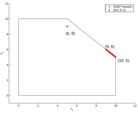
Example 2. Consider a modification of Example 1 where the shared constraint x ₁ + x ₂ ≤ 1 is changed to x ² ₁ + x ² ₂ ≤ 1. It can be seen that the GNEs are the vectors

x ₁ x ₂

= √ t

1 − t ²

, 0 ≤ t ≤ ⁴ ₅ .

The corresponding VI (F, X) still has only one solution since F is unchanged and remains strongly monotone. At the GNE x = (0, 1) ^T , M(x) = ∅ (due to the constraint x ² ₁ ≤ 0 in the problem of player 1). Thus the approach of Section 3.1 would not find this GNE.

The shared constraint function in Example 2 is separable, which we will exploit in developing our primal, or resource-directed, parametrization. Specifically, we make the following blanket assumption in this subsection.

Assumption C. The shared constraint function g has the form (10), where g ˆ _ν = (ˆ g _ν,i ) ^m _i=1 ^¯ : ⁿ

→ ^{m ¯} , ν = 1, . . . , N , and each ˆ g _ν,i is a differentiable convex function.

Now, we construct a family of VIs that contains VI (F, X) as a particular instance. Let β = (β _ν ) ^N _ν=1 ∈ ^m with β _ν ∈ ^{m ¯} , ν = 1, . . . , N, be a vector of parameters satisfying _N

ν=1 β _ν = 0.

Define the set X ^β ⊂ X by

X ^β := X ₁ ^β

× · · · × X _N ^β

with X _ν ^β

:= { x _ν ∈ X _ν | g ˆ _ν (x _ν ) ≤ β _ν } , ν = 1, . . . , N,

and consider VI (F, X ^β ). By Assumption C, X ^β is closed and convex (possibly empty). In- tuitively, we parametrize the division of resources among the players, reminiscent of Bender’s decomposition.

Now, we investigate the relationship between VI (F, X ^β ) and GNEP. The following result is

easy to see.

Theorem 3.5. For any GNE x

, we have x

∈ SOL (F, X ^β ) and _N

ν=1 β _ν = 0, where we let β _ν = ˆ g _ν (x

_ν ) − α _ν g(x

) with arbitrary real numbers α _ν such that _N

ν=1 α _ν = 1 and α _ν > 0, ν = 1, . . . , N.

Corollary 3.3.

P_N

ν=1

β

=0

SOL (F, X ^β ) ⊃ SOL

.

In Example 2, if we choose ˆ g ₁ (x ₁ ) = x ² ₁ and ˆ g ₂ (x ₂ ) = x ² ₂ − 1, then SOL (F, X ^β ) =

(0, 1) ^T for β = (0, 0) ^T . In general, VI (F, X ^β ) need not have a solution or a solution need not be a GNE.

The next result gives a sufficient condition for a solution of VI (F, X ^β ) to be a GNE.

Theorem 3.6. For any β ∈ ^m with _N

ν=1 β _ν = 0 and any x

∈ SOL (F, X ^β ), a sufficient condition for x

to be a GNE is that

for each i = 1, . . . , m, ¯

either g ˆ _ν,i (x

_ν ) = β _ν,i ν = 1, . . . , N or g ˆ _ν,i (x

_ν ) < β _ν,i ν = 1, . . . , N.

(14) Proof. Since x

is a solution of VI (F, X ^β ), for each ν = 1, . . . , N, we have that x

_ν is a solution of VI ( ∇ _x

θ _ν ( · , x

), X _ν ^β

) or, equivalently, x

_ν is an optimal solution of the convex programming problem:

minimize θ _ν (x _ν , x

)

subject to x _ν ∈ X _ν , ˆ g _ν (x _ν ) ≤ β _ν . (15) By (14) and Assumption C, for each i, we have either ˆ g _ν,i (x

_ν ) = β _ν,i = −

ν

β _ν

,i = −

ν

ˆ g _ν

,i (x

_ν

), implying g _i (x

) = 0, or ˆ g _ν,i (x

_ν ) < β _ν,i = −

ν

β _ν

,i < −

ν

g ˆ _ν

,i (x

_ν

), implying g _i (x

) < 0.

Thus, for each ν, x

_ν is also an optimal solution of the problem:

minimize θ _ν (x _ν , x

)

subject to x _ν ∈ X _ν , g(x _ν , x

) ≤ 0. (16) In particular, the active inequality constraints at x

_ν in (15) coincide with those in (16). In view of Assumption B and (3), the above problem is exactly P _ν (x

). This shows that (2) holds and hence x

is a GNE.

Notice that, for any GNE x

, the β given in Theorem 3.5 satisfies the sufficient condition (14).

Thus, we can refine Corollary 3.3 to

PN ν=1βν=0

(14) holds for some x∗∈SOL (F,Xβ)

SOL (F, X ^β ) ⊃ SOL

.

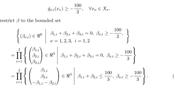
If there exist a _ν ∈ ^{m ¯} , ν = 1, . . . , N , such that ˆ

g _ν (x _ν ) ≥ a _ν , ∀ x _ν ∈ X _ν , ν = 1, . . . , N, then we can further restrict β to the bounded set

β ∈ ^m

N ν=1

β _ν = 0, β _ν ≥ a _ν , ν = 1, . . . , N

.

In Example 2, if we choose ˆ g ₁ (x ₁ ) = x ² ₁ and ˆ g ₂ (x ₂ ) = x ² ₂ − 1, then we can take as lower bounds

a ₁ = 0 and a ₂ = − 1.

If a solution x

of VI (F, X ^β ) has a Lagrange multiplier λ

_ν associated with each constraint ˆ

g _ν (x _ν ) ≤ β _ν , i.e., 0 ≤ λ

_ν ⊥ g ˆ _ν (x

_ν ) − β _ν ≤ 0, then letting π

= min

ν=1,...,N λ

_ν , Δ _ν = λ

_ν − π

, ν = 1, . . . , N,

where the “min” is taken componentwise, we see that (x

, π

) satisfies the KKT condition (11) for VI (F ^Δ , X). Thus, VI (F ^Δ , X) may be viewed as the dual of VI (F, X ^β ), with the former requiring separability of shared constraints and the latter requiring a CQ to ensure existence of Lagrange multipliers.

3.3 Relation between some GNE concepts and VI approaches

In this subsection, we discuss the normalized equilibrium introduced by Rosen [23] in relation to the solution sets obtained by the VI approaches discussed in the previous subsections. We make the following assumption through this subsection.

Assumption D. A suitable CQ holds at every GNEs.

Assumption D implies that for every GNE x

there exists a Lagrange multiplier λ

= (λ

_ν ) ^N _ν=1 ∈ ^m that satisfies the KKT system (5).

The normalized equilibrium is defined as follows [23]:

Definition 3.2. Let a GNE x

together with a Lagrange multiplier λ

= (λ

_ν ) ^N _ν=1 ∈ ^m satisfies the KKT system (5). We call x

a normalized equilibrium if there exists vectors r ∈ ^N ₊₊ and λ ∈ ^m such that

λ

_ν = λ/r _ν ν = 1, . . . , N.

Rosen [23] proves that there exists a normalized equilibrium for any given r = (r _ν ) ^N _ν=1 ∈ ^N ₊₊ if the set X is compact. He defines the weighted Nikaido-Isoda-type function ρ : ⁿ × ⁿ × ^N → by

ρ(x, y, r) = N ν=1

r _ν θ _ν (x ₁ , . . . , y _ν , . . . , x _N ), and shows that there exists a point x

∈ X such that

ρ(x

, x

, r) = max

y∈X { ρ(x

, y, r) } (17)

to establish the existence of a normalized equilibrium. Note that it is easy to see that the KKT condition for (17) is equivalent to the KKT condition for the VI ( ˜ F ^r , X) where ˜ F ^r : ⁿ → ⁿ is given by

F ˜ ^r (x) = (r _ν ∇ _x

θ _ν (x)) ^N _ν=1 . Rosen’s results may be summarized with our notation as follows.

Theorem 3.7. [23, Theorem 3] For each r ∈ ^N ₊₊ , any solution of VI ( ˜ F ^r , X) is a normalized equilibrium.

Theorem 3.8. [23, Theorem 4] Assume that X is bounded and F ˜ ^r is strictly monotone for every

r ∈ Q, where Q is a subset of ^N ₊₊ . Then there is a unique normalized equilibrium for each r ∈ Q.

Note that the monotonicity of F does not imply the monotonicity of ˜ F ^r . In fact, consider the mapping F : ² → ² defined by

F (x ₁ , x ₂ ) = 2x ₁ + x ₂ x ₁ + 2x ₂

is monotone. However, a mapping ˜ F ^r : ² → ² with weight (r ₁ , r ₂ ) = (15, 1) is given by F ˜ ^r (x ₁ , x ₂ ) = 30x ₁ + 15x ₂

x ₁ + 2x ₂

,

which is not monotone because for vectors x = (1, − 4) and y = (0, 0) we have F ˜ ^r (x) − F ˜ ^r (y), x − y = − 2 < 0.

Now we investigate the difference between normalized equilibrium and GNE, and besides, we discuss the relation with the solution set of the VI formulations. Below, the set of normalized equilibria is denoted by SOL ^N .

From the definition of these concepts among with Theorems 3.1, 3.7 and Corollary 3.1, we have the following relation:

SOL (F, X)

⊆

SOL ^N =

r∈

SOL ( ˜ F ^r , X)

⊆ ⊆

SOL

⊆

Δ∈

SOL (F ^Δ , X).

For any (x, λ) satisfying the KKT system (5), we say strict complementarity holds at (x, λ) if g _i (x) = 0 implies λ _ν,i > 0 for any ν = 1, . . . , N and i = 1, . . . , m.

The next proposition states that, when there is only one shared constraint, all GNE are nor- malized equilibrium as long as the strict complementarity holds.

Proposition 3.2. Suppose that there is only one shared constraint and assume that M (x

) = ∅ for every GNE x

. If strict complementarity holds at (x

, λ

) for every GNE x

and some λ

∈ M (x

), then every GNE x

is a normalized equilibrium.

Proof. If the shared constraint is inactive, i.e., g(x

) < 0, then we have λ

_ν = 0, ν = 1, . . . , N and it is obvious that x

is a normalized equilibrium.

Suppose that g(x

) = 0. Then it implies λ

_ν > 0 for all ν by the strict complementarity assumption. Let λ ∈ and a weight vector r ∈ ^N be given by

λ := 1 r _ν := 1

λ

_ν , ν = 1, . . . , N.

Then we have λ

_ν = _r ^λ

ν

for ν = 1, . . . , N . This indicates that x

is a normalized equilibrium.

Corollary 3.4. Suppose that the assumptions of Proposition 3.2 hold. Then we have

r∈

SOL ( ˜ F ^r , X) = SOL ^N = SOL

,

and hence the following relation holds:

SOL (F, X)

⊆

SOL ^N =

r∈

SOL ( ˜ F ^r , X)

= ⊆

SOL

⊆

Δ∈

SOL (F ^Δ , X).

From the above results, in the single shared constraint case, we may expect to obtain all GNE by means of parametrization with weights r _ν on the objective functions θ _ν .

In the case of multiple shared constraints, however, such parametrization may fail to yield the set of GNE, since a GNE is not necessarily a normalized equilibrium in general. This is illustrated in the next example.

Example 3. Consider the following two-person game, where player 1 and player 2 solve the minimization problems

P ₁ (z) : minimize

x,y x ² + xy + y ² + (x + y)z − 25x − 38y subject to x ≥ 0

y ≥ 0

x + 2y − z ≤ 14 3x + 2y + z ≤ 30, P ₂ (x, y) : minimize

z z ² + (x + y)z − 25z subject to z ≥ 0

x + 2y − z ≤ 14 3x + 2y + z ≤ 30, respectively. This is a GNEP with two shared constraints.

The solution set of this GNEP consists of vectors

⎛

⎝ x y z

⎞

⎠ =

⎛

⎝ t 11 − t

8 − t

⎞

⎠ , t ∈ [0, 2].

Hence the shared constraints are both active at each GNE.

Note that the VI (F, X) has a single solution

⎛

⎝ x y z

⎞

⎠ =

⎛

⎝ 0 11

8

⎞

⎠ .

The Lagrange multipliers λ = (λ _ν,i ) ∈ ⁴ corresponding to the GNE (x(t), y(t), z(t)) = (t, 11 − t, 8 − t) is given by

⎛

⎜ ⎜

⎜ ⎝ λ _1,1 (t) λ _1,2 (t) λ _2,1 (t) λ _2,2 (t)

⎞

⎟ ⎟

⎟ ⎠ =

⎛

⎜ ⎜

⎜ ⎝

3 2 t + 3 1 − ₂ ^t s + 2 − 2t

s

⎞

⎟ ⎟

⎟ ⎠ , s ≥ max { 0, 2t − 2 } .

Thus the tuple (λ ₁ , λ ₂ , r ₁ , r ₂ ) ∈ ⁴ ₊ satisfying λ ₁

r ₁ = λ _1,1 (t), λ ₂

r ₁ = λ _1,2 (t), λ ₁

r ₂ = λ _2,1 (t), λ ₂

r ₂ = λ _2,2 (t)

exists only if 0 ≤ t < 1. Hence, the following relation holds in this example:

⎧ ⎨

⎩

⎛

⎝ 0 11

8

⎞

⎠

⎫ ⎬

⎭ = SOL (F, X)

⎧ ⎨

⎩

⎛

⎝ t 11 − t

8 − t

⎞

⎠

0 ≤ t < 1

⎫ ⎬

⎭ = SOL ^N

⎧ ⎨

⎩

⎛

⎝ t 11 − t

8 − t

⎞

⎠

0 ≤ t ≤ 2

⎫ ⎬

⎭ = SOL

.

This example indicates that, when there are more than one shared constraints, some GNE may not be obtained by the VI approach using parametrization with weights on the objective functions.

4 Numerical Experiments

In this section, we show some numerical experiments with our VI approaches. We give a brief description of the GNEPs taken from the literature in the next subsection and present numerical results of our approaches in Subsection 4.2.

4.1 Examples

Example 4 (Harker’s example). This problem is taken from [8]. There are two players and they solve the following problems:

P ₁ (x ₂ ) : minimize x ² ₁ + ⁸ ₃ x ₁ x ₂ − 34x ₁ subject to 0 ≤ x ₁ ≤ 10

x ₁ + x ₂ ≤ 15,

P ₂ (x ₁ ) : minimize x ² ₂ + ⁵ ₄ x ₁ x ₂ − 24.25x ₂ subject to 0 ≤ x ₂ ≤ 10

x ₁ + x ₂ ≤ 15.

This is a GNEP with one shared constraint and the solution set is given by SOL

= 5

9

∪ t

15 − t

9 ≤ t ≤ 10

. (18)

The corresponding F : ² → ² and X ⊆ ² are represented as F (x) = 2x ₁ + ⁸ ₃ x ₂ − 34

5 4 x ₁ + 2x ₂ − 24.25

, (19)

X =

x ∈ ² | x ₁ + x ₂ ≤ 15, 0 ≤ x _ν ≤ 15, ν = 1, 2 .

Since F is strongly monotone on ² , VI (F, X) has a unique solution, which is given by x = (5, 9) ^T . Note that this solution lies in the interior of the set X.

Example 5 (River basin pollution game). Consider the 3-person river basin pollution game studied in [13, Section 5.3], where the problem of player ν ∈ { 1, 2, 3 } is defined by

P _ν (x _ν ) : minimize (α _ν x _ν + β(x ₁ + x ₂ + x ₃ ) − χ _ν )x _ν subject to x _ν ≥ 0,

3.25x ₁ + 1.25x ₂ + 4.125x ₃ ≤ 100,

2.2915x ₁ + 1.5625x ₂ + 2.8125x ₃ ≤ 100,

with α ₁ = 0.01, α ₂ = 0.05, α ₃ = 0.01, β = 0.01, χ ₁ = 2.9, χ ₂ = 2.88, χ ₃ = 2.85. This GNEP has two shared constraints. The corresponding F : ³ → ³ and X ⊆ ³ are given by

F (x) =

⎛

⎝ 0.04 0.01 0.01 0.01 0.12 0.01 0.01 0.01 0.04

⎞

⎠ x −

⎛

⎝ 2.9 2.88 2.85

⎞

⎠ , (20)

X =

x ∈ ³ ₊

3.25 1.25 4.125 2.2915 1.5625 2.8125

x ≤ 100 100

.

Since F is strongly monotone on ³ , VI (F, X) has a single solution, which given by x = ( ⁴⁶⁷³ ₂₂₁ , ⁵⁷⁵⁴ ₃₅₉ , ⁵⁶⁷ ₂₀₈ ) ^T ≈ (21.14, 16.03, 2.73) ^T . Note that, at this solution, the first inequality defin- ing X is active, while the second inequality is inactive.

Example 6 (Electric power market model). We take a model in electric power markets with endogenous arbitrage from [19, Section 5.3]. The model consists of several electricity firms competing on a spatial network of markets along with an arbitrager who attempts to make a profit by exploiting price differentials between regions. In the original model [11], each firm maximizes its profit with anticipating the arbitragers’ optimal response, resulting in a multi-leader-follower- game. In [19, Section 5.3], the arbitrager is removed from the model and the price differentials are assumed to be less than the shipping costs. In this setting, the model can be formulated as a GNEP as described in the following.

The regions are represented by the nodes in a network and each firm has electric plants at those nodes. Each firm determines how much it should produce at each plant and how much it should sell at each node to maximize its profit.

We introduce the notations to formulate the problem.

Parameters

N : set of nodes F : set of firms

c ^f _i : cost per unit generation at node i by firm f P _i : price intercept of sales function at node i Q _i : quantity intercept of sales function at node i e _ij : unit cost of shipping from node i to j

CAP ^f _i : production capacity at node i for firm f Variables

s ^f _ij : amount produced at node i and sold at node j by firm f S _j : amount of total sales at node j

S _j :=

t∈F

i∈N

s ^t _ij , ∀j ∈ N p _j : market price at node j

p _j (S _j ) := P _j − P _j

Q _j S _j , ∀j ∈ N

Each firm f ’s problem is to find s ^f _ij , (i, j) ∈ N × N that solve the following maximization