修士論文概要(2019年2月) 京都大学大学院工学研究科 都市社会工学専攻
Quasi-dynamic network assignment model with public transport and competition for free floating bicycles
姚 子昴1*
*交通マネジメント講座 交通情報工学分野
1.Background
Although the idea of ‘free floating’ is rather new, free floating bicycle services (FFBS, also called stationless, dockless or station- free), have boomed on the street since 2015, thanks to the rapid expansion of dozens of private start- up companies in China and around the world. The new free- floating mode provides users more flexible choices because it allows users to start and end their trip much closer to their true origin and destination, compared to the conventional station based bikesharing. The hardware on the free-floating bicycles has evolved into second generation, which now integrated with global positioning systems (GPS) modules and Bluetooth communications modules. These characteristics have enabled the service providers to gather the time and GPS location information of each travel, and even may be able to record the GPS path of each travel. This system has the potential to become a rich mine of robust travel data.
2. Objective
In our quasi-dynamic model, with given initial bicycle density and OD demand in this time interval, we firstly proposed a closest-bicycle seeking process universally feasible for any distribution under Euclidean distance, to generate the travel cost function for each mode. Based on the travel cost function, incremental assignment is used to assign OD demand among different modes. The volume information on each mode in time N can be used to update the initial bicycle distribution for time interval N+1. For the building of a quasi-dynamic distribution forecast model, we conduct the research processes in each individual time interval.
3. Overall framwork We firstly define:
𝐿, 𝐼: set of links, nodes describing then transport network
𝜑𝐴(𝑡): initial distribution of FFBS at time 𝑡 in area 𝐴 𝑔𝑖𝑗(𝑡): demand from 𝑖 to 𝑗 in time interval 𝑡
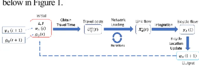
𝑈𝑖𝑗𝑚(𝑡): utility of mode 𝑚 from 𝑖 to 𝑗 in time interval 𝑡 𝑋𝑎∗(𝑡): the equilibrium link flow pattern in time interval 𝑡 𝑦𝐴(𝑡): the net bicycle flow at 𝑋𝑎∗(𝑡) between areas At each time interval 𝑡 , the expected process is shown
below in Figure 1.
Figure 1 Quasi-dynamic distribution forecast model
The abstraction from PT service in the research area to the PT network is firstly done before any interval starts. At the beginning of each interval, we firstly provide the bicycle distribution at the beginning of this interval, 𝜑𝐴(𝑡), and the travel demand during this interval, 𝑔𝑖𝑗(𝑡) , as input. By invoking the closest-bicycle-seeking process, which will be introduced in the next section, the travel time of each mode can be calculated. Based on the travel time, the utility of each mode can be acquired. By applying a stochastic network loading approach, the link flow pattern will be generated. The area flow is the aggregation of the inbound flow and outbound flow of each zone. By integrating the initial bicycle distribution and the area flows, we can update the final state bicycle distribution pattern as the output of this interval, also served as the initial bicycle distribution, 𝜑𝐴(𝑡 + 1) at interval 𝑡 + 1 . This updated bicycle distribution together with the travel demand of the next interval can again serve as the input for next loop.
4. Methods
Order statistics is adopted to represent the the randomized characteristics of free-floating bicycle-sharing in the form of link cost. We follow the simple definition given by H.A.David and H.N.Nagaraja (2004):
If the statistically IID random variables 𝑋1, … , 𝑋𝑛 are arranged in order of magnitude and then written as 𝑋(1)≤
⋯ ≤ 𝑋(𝑛), we call 𝑋(𝑖) the 𝑖𝑡ℎ order statistic (𝑖 = 1, … , 𝑛).
Correspondingly, the 1𝑠𝑡 order statistic is the minimum value of the sample, and the 𝑛𝑡ℎ order statistic is the maximum value when the sample size is 𝒏.
Let 𝑋1, … , 𝑋𝑛 be random variables, and order statistic 𝑌(1)= ℎ1(𝑋1, … , 𝑋𝑛), ,, 𝑌(𝑘) = ℎ𝑘(𝑋1, … , 𝑋𝑛) be an 1-1 transformation, with 𝑥1= 𝑤1(𝑦(1), … , 𝑦(𝑛)), ,,
修士論文概要(2019年2月) 京都大学大学院工学研究科 都市社会工学専攻
𝑥𝑘= 𝑤𝑘(𝑦(1), … , 𝑦(𝑛)) be the inverse functions. The joint pdf of 𝑌(1) to 𝑌(𝑘) is:
𝑓(1,… ,𝑘)(𝑦1, … , 𝑦𝑘) = 𝑓[𝑤1(𝑦1, … , 𝑦𝑛), … , 𝑤𝑘(𝑦1, … , 𝑦𝑛)]|𝐽|
which |𝐽| is the determinant of the Jacobian matrix. The general form of the joint pdf of 𝑌(1)to 𝑌(𝑘)is:
𝑓(1,… ,𝑘)(𝑦(1), … , 𝑦(𝑘)) = 𝑛! ∏ 𝑓(𝑦(𝑘))
𝑘=𝑛 𝑘=1
The marginal pdf of 𝑌(𝑗) with sample size 𝒏 is:
𝑓(𝑗)(𝑦(𝑗)) = 𝑛!
(𝑗 − 1)! (𝑛 − 𝑗)![𝐹(𝑦(𝑗))]𝑗−1[1 − 𝐹(𝑦(𝑗))]𝑛−𝑗𝑓(𝑦(𝑗))
5. Case setting
We tested several different demand patterns and supply patterns in our research. These cases can be shown as:
{One day, N day} scenarios
× {symmetric, asymmetric} demand
× {with, without} noon interval
× {with, without} periphery flow
Together with uniform demand scenario and another three propagation scenarios each starts from one specific zone.
The evaluating criteria in this research are the total travel time, 𝑇𝑡𝑜𝑡𝑎𝑙, and the bicycle supply pattern, (𝐵𝐴, 𝐵𝐵, 𝐵𝐶).
6. Results and Conclusions
We categorize the results and conclusions into three groups.
1. Microcosmically
The bicycles in CDB area are ‘diluted’ into surroundings during evening peak. This ‘dilution effects’ is widely observed. This phenomenon can be explained as the easier access to bicycles in highly condensed area.
Comparing the surrounding zones, bicycles tend to flow to smaller zone. This ‘minority paradox’ is also tested and explained. Generally speaking, such paradox disappears when such zone is too small.
2. One-day Scenario
Asymmetric scenarios generally have worse performance in total travel time. This can be explained as more condensed demand in a specific zone will generally worsen the experience of all other travelers in this network because of the more intensive competitions.
The introduction of noon interval does not change the optimal supply pattern. Even with the existence of periphery flows, the optimal pattern is also acceptable with the maximum at 16.7% worse, which suggests analyzing major flows in morning and evening peak can also provide a modest approximation.
3. N-day Scenario
The fluctuation patterns are oscillation convergent in each scenario. Separately introducing noon interval or periphery flows may not lead to a faster convergence. The joint influence of noon interval and periphery flows will make the network more stable and faster to converge.
The supply pattern at equilibrium is different from the minimal total travel time pattern. We do not agree this can be explained as some transformation of Braess's paradox.
The bicycle supply is changed after each iteration, thus will cause the bicycle supply pattern to change. The changes in the supply pattern will automatically influence the formation of link cost functions. Together we can find out that the network structure is altered after each iteration.
8. Further studies
This research can be further expanded and modified in the following topics.
1. Evaluate accessibility influence of rebalancing In order to develop a better initial supply pattern with less rebalancing demand but still maintain a high level of usage rate
2. Evaluate fleet size
In order to obtain balance between service level and fleet size thus bicycles as carefully regulated.
3. From quasi-dynamic to real-time
In order to provide more reasonable and realistic outcomes such as evaluating long-time travels.
4. From uniform distribution to more realistic distributions
In order to simulate bicycles accumulating around PT stations, such as adopting Rayleigh Distribution.
5. Real-world scale methodologies
To avoid O(𝑛2 ) time complexity of the current approach and numerical approaches and approximations are essential.
Reference
Philip, J. (2007). The probability distribution of the distance between two random points in a box.
H.A.David, & H.N.Nagaraja. (2004). Order Statistics (3rd edition). In (Vol. 9): Encyclopedia of Statistical Sciences.
修士論文指導教員
山田忠史 教授, Jan-Dirk Schmoecker 准教授, 藤井聡 教授