Distributed Estimation over Delayed Sensor Network with Scalable Communication

(1)

PAPER

Distributed Estimation over Delayed Sensor Network with Scalable Communication

Ryosuke ADACHI^†a),Nonmember, Yuh YAMASHITA^†,andKoichi KOBAYASHI^†,Members

SUMMARY This paper proposes a distributed delay-compensated observer for a wireless sensor network with delay. Each node of the sensor network aggregates data from the other nodes and sends the aggregated data to the neighbor nodes. In this communication, each node also compensates communication delays among the neighbor nodes. Therefore, all of the nodes can synchronize their sensor measurements using scalable and local communication in real-time. All of the nodes estimate the state variables of a system simultaneously. The observer in each node is similar to the delay- compensated observer with multi-sensor delays proposed by Watanabe et al. Convergence rates for the proposed observer can be arbitrarily designed regardless of the communication delays. The effectiveness of the proposed method is verified by a numerical simulation.

key words: sensor network, data aggregation, communication delay, distributed estimation

1. Introduction

Sensor networks with numerous sensors have attracted much attention because the development of micro-electro- mechanical systems (MEMS) has improved the perfor- mance of compact sensors and communication elements[1].

Many sensors can realize a wide-range of complex obser- vations in large-scale systems. Redundant sensors improve the accuracy and robustness of an observation, and enable a fault-tolerant observation. A flexible sensing system can be realized by connecting sensors via a wireless network. Such a sensor network can be used in various applications, includ- ing area surveillance or the active monitoring of forests and agricultural lands.

There have been many studies on the applications of sensor networks [2]–[9]. Distributed estimation methods have also been proposed to reduce wasteful communication paths. Olfati-Saber et al. [10]–[13] proposed a distributed Kalman filter based on a consensus filter. The consensus filter is an application of consensus controls, and pro- vides the average consensus of all the sensors included in a network. The consensus filter can calculate the consensus value through communications between adjacent nodes. An estimate of the distributed Kalman filter is obtained from the original Kalman filter using the consensus value [14].

Olfati-Saber et al. also proposed a Kalman-consensus filter, which executes the Kalman filtering and consensus calculation simultaneously. A gossip algorithm is also a distributed

Manuscript received July 19, 2018.

Manuscript revised January 12, 2019.

†The authors are with Hokkaido University, Sapporo-shi, 060- 0814 Japan.

a) E-mail: [email protected] DOI: 10.1587/transfun.E102.A.712

consensus algorithm for sensor networks[15]. In the gossip algorithm, each node selects the data sent from the other nodes at random. This reduces the communication traffic of the sensor network, and allows this algorithm to obtain a consensus value.

These studies focus on the communication efficiency.

The communication delay is another problem of a sensor network with delay. In particular, the communication delays in a large wireless network cannot be ignored. However, the distributed estimation methods discussed in previous studies do not consider the communication delay. Delay compensated observers, which do not assume a network structure, have been proposed in[16]–[18]. In particular, Watanabe et al.[16]and Tsubakino et al.[18]considered the case where the output vector includes multiple delays. The delays included in the network are non-uniform, because they depend on the communication paths. The design of Watanabe’s observer resolves itself into a finite pole assignment problem.

In this paper, we bring a network structure to Watan- abe’s delay-compensated observer. A distributed estimation method with delay compensation is proposed here. Watan- abe defined an output vector, where each element of the vector is a sum of multiple measurements of a physical quantity with different delays. The output form of Watanabe’s observer is useful in aggregating the observed values using distributed data aggregation methods. Data aggregation methods for a sensor network are proposed in[19]. In this paper, we introduce the delay compensation proposed in [16]for tree-based data aggregation. All of the observed values of the sensor network are aggregated through communications between the neighbor-node pairs in a tree network. The observed values of the sensor network are aggregated by the tree-based communication at the root node. The communication delays are compensated by the memory of the input stored by each node. An observer of the root node can estimate the state from the aggregated data at its own node. We also propose an intercommunication protocol to aggregate the observed values in all the nodes, which is based on the fact that each node of a tree network can be a root node. Fi- nally, the distributed observer can estimate the states at all the nodes. A dimension of the communication data among the nodes corresponds to a dimension of the output vector.

Because the dimension of the output vector is independent of the number of nodes, the proposed communication law in this paper is scalable.

Copyright c2019 The Institute of Electronics, Information and Communication Engineers

(2)

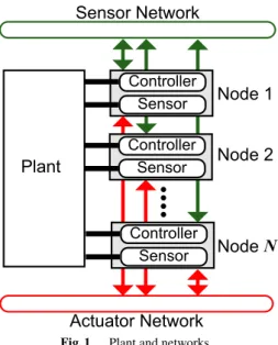
Fig. 1 Plant and networks.

2. Problem Formulation

Figure 1 shows a system with distributed controllers. The dynamics of the plant in Fig. 1 can be expressed by

˙

x=Ax+Bu, (1)

wherex∈Rⁿis the system state, andu∈R^mrepresents the input values of the distributed controllers. Some states of system (1) can be measured by sensors as

y=C x, (2)

wherey ∈R^p is an output vector that consists of all of the redundant raw measurements, and therefore rankCmay be less than p, and pmay be larger thann. For the scalability of the network communication with respect to the number of sensors, this paper considers aggregations of sensor measurements. To reduce a communication amont, we utilize a data aggregation of the measurements. The raw outputyis aggregated into aq-dimensional vectoryagras

y_agr =Fy=Cagrx, (3)

whereCagr = FC. Note that q < p because the data aggregation reduce the dimension of original outputy. The designs ofF andq are important because these affect the performances of the state estimation or control, as indicated in[20]. However, this paper focuses on other problems, and we assume thatFis given.

There are two networks in Fig. 1, i.e., a sensor network and an actuator network that share the same node set with N elements. Each node may have the sensors and a controller. Each controller collects the observed information from the other nodes via the sensor network to estimate the statex, and calculates a part of the input elements from the estimated value. By renumbering the elements ofy, we can decompose matrixFas

=

whereFicorresponds to the output of thei-th node. There- fore, the output of nodei, which is mapped to the aggregated output space, is defined as

y1= F1 0 · · · 0 y=C1x ...

y_N = 0 · · · 0 F_N y=CNx,

(4)

whereC_i = 0 · · · 0 Fi 0 · · · 0 C. If the current outputsyican be obtained with no transmission delay, the aggregated output coincides withy_agr, i.e.

y_agr =

N

X

i=1

y_i. (5)

Each node needs all of the input values to estimate the state. In this paper, it is assumed that the dimension of the input is smaller than that of the output. Each node sends the input values via a high-speed actuator network with a lim- ited capacity. On the other hand, the observed values of each of the nodes are sent via a sensor network with sufficient bandwidth but low communication speed. Therefore, the communication delay in the transmission of the input values is sufficiently smaller than that for the observed values.

We have ignored the communication delay in the broadcast of the input values, and it is assumed that all the nodes can obtain the input instantly.

We represent the sensor network by an undirected graph. The set of nodes is denoted by V := {1,2, ....,N}, and the set of edges is denoted by E ⊆V×V. By usingV andE, the undirected graph is expressed byG(V,E). In this paper, it is assumed that the graphGis a connected graph.

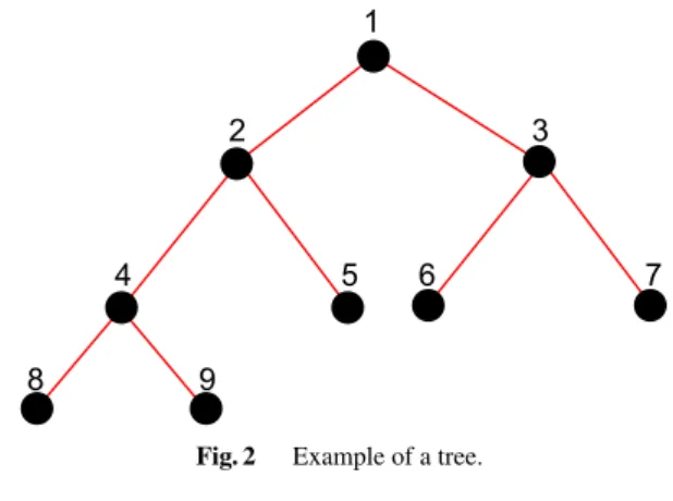
For the connected graphG, there always exists at least one tree that is a subgraph ofGand includes all the nodes ofV.

This tree is denoted byT(V,E), where ˆˆ E satisfies ˆE ⊆ E.

Nodeican mutually communicate with the neighbor nodes.

The set of neighbors of nodeiconnected byT is denoted by Ji:={j; (i,j)∈E}. Once a root node of the undirected treeˆ is chosen, the parent node and child nodes of each node are automatically determined. A set of the child nodes of nodei is denoted byHir, where ther-th node is chosen as the root node. From the definition H_ir andJ_i, H_ir ⊆ J_i. If r = i, Hir = Ji. Otherwise,{pir} = Ji\Hir, wherepiris a parent node of nodeiwhenris the root. For example, the set of child nodes of node 4 in Fig. 2 is

H2r=











{1,4,5} ifr=2 {1,5} ifr=4,8,9 {1,4} ifr=5 {4,5} ifr=1,3,6,7

.

A communication delay from node jtoiis denoted byDi j. If j<Ji,Di jbecomes the total delay in the path from node jtoi. For example,D81 of the tree in Fig. 2 isD81 =D84+

(3)

Fig. 2 Example of a tree.

D42+D21.

Remark 1. In many cases, it is assumed thatDi j = Dji, which is a natural assumption. However, the method proposed in this paper does not need this assumption.

Remark 2. The sensor network may have relay nodes. A relay node does not have a sensor but can communicate with the other nodes. The output matrix of the relay node isCi= 0. Several systems can be realized using relay nodes. For example, a system with a single centralized controller can be expressed by a network that includes a controller and has a relay node as the root node.

Main problems in this paper is design a consensus communication law for distributed observer over delayed sensor networks. For the communication and estimation, nodei hasΛi := {A,B,{Di j;j ∈ Ji},Ci,Cˆi,{C¯i j;j ∈ Ji}} in own memory, where ˆCi and ¯Ci j will be defined in Sects. 3.2 and 3.3. From the actuator network, the all nodes can obtain u(t) in real-time and store the history of input u(τ),

τ ∈ [t,t−Di,max], where Di,max is the maximum delay ex-

pressed byDi,max =maxj∈J_iDi j. To simplify the problem, we divide the problem into the following two parts. In Prob- lem 1, the rootris fixed and each node sends a message to own parent node. The message sent to the parent node by nodeiis{ˆyi(t),Ξˆi(t)}, where ˆyi(t) is an aggregate measure- ment and ˆΞi(t) is a compensation value for communication delays. Then, only the root estimates the state as follows:

Problem 1. Assume that noderis fixed as the root node of T and (A,Cˆr) is the observable pair. GivenΛifor alli∈V. Then, find the communication law

yî(t)=gî(yi,{ˆyj(t−Di j);j∈Hir}), Ξî(t)=hî({Ξˆj(t−Di j);j∈Hir},

{u(τ);t−Di,max≤τ≤t}), and the observer in the root

˙ˆ

xr(t)=fr( ˆxr(t),u(t),yˆ_r(t),Ξˆr(t)), such that

t→∞lim(x(t)−xˆr(t))=0.

In Problem 2, the messages received from the neighbor nodes by node i are {¯yi j(t),Ξ¯i j(t)}(j ∈ Ji). Then, the all nodes estimate the state as follows:

Problem 2. Assume that (A,Cˆi) for alli∈Vare the observable pairs. GivenΛifor alli∈V. Then, find the communication law

y¯i j(t)=g¯i j(yi,{y¯ki(t−Dik);k∈Ji}), Ξ¯i j(t)=h¯_{i j}({Ξ¯ki(t−D_ik);j∈J_i},

{u(τ);t−D_i,max≤τ≤t}),

and the distributed observers

yˆ_i(t)=gˆ_i(y_i,{y¯_ki(t−D_ik);k∈J_i})), Ξˆi(t)=hˆi({Ξ¯ki(t−Dik);j∈Ji},

{u(τ);t−Di,max≤τ≤t}),

˙ˆ

xr(t)= fr( ˆxr(t),u(t),yˆ_r(t),Ξˆr(t)), such that

t→∞lim(x(t)−xˆi(t))=0.

We will obtain a result for Problem 1 in Sect. 3.2, and then extend it to Problem 2 in Sect. 3.3.

3. Proposed Method

3.1 Preliminary

In this subsection, the past work which will be utilized for a delay compensation in the proposed method is introduced.

The data received at each node includes multiple delays because the communication delays in the sensor network depend on the selection of communication paths. An observer with multi-sensor delays was proposed in[16]. Watanabe et al.[16]defines the outputsCixfor each corresponding delay Di. Thus the output from all the measurements is expressed by

ycen(t)=

N

X

i=1

Cix(t−Di). (6)

We can compensate the delays in (6) by predicting the system behavior.

Lemma 1 (Delay-Compensation Based on Prediction).

Consider system (1) with output (6). For this system, the following equation holds:

ycen(t)+

N

X

i=1

Cie^−ADⁱ Z t

t−D_i

e^A(t−τ)Bu(τ)dτ=C x(t),ˆ (7) where ˆC=PN

i=1Cie^−ADⁱ.

(4)

x(t)=e^ADⁱx(t−Di)+Z t t−Di

e^A(t−τ)Bu(τ)dτ. (8)

Lemma 1 can be proven by solving (8) with respect tox(t−

D_i) and inserting it into (6).

From Lemma 1, the state estimation for the system (1) with (6) becomes a finite pole assignment problem as follows.

Lemma 2(Watanabe’s Delay-Compensated Observer[16]).

Consider system (1), the output (6), and the observer

˙ˆ

x(t)=Ax(t)ˆ +Bu(t) +L





 y_cen(t)+

N

X

i=1

Cie^−ADⁱ Z t

t−Di

e^A(t−τ)Bu(τ)dτ

−

N

X

i=1

Cie^−ADⁱx(t)ˆ





,

(9)

and suppose that (A,C) is an observable pair. Then, the es-ˆ timation error ˜x = x−xˆconverges to zero, if and only if A−LCˆis Hurwitz.

Proof. From Lemma 1, the dynamics of ˜xcan be expressed by

˙˜

x=(A−LC) ˜ˆ x. (10)

Therefore, ˜xtends to zero ast→ ∞if and only ifA−LCˆis

Hurwitz.

We notice that Watanabe’s delay-compensated observer does not need to handley, as defined by (2). The single output vector ycen defined by (6), which includes all the delayed sensor signals, and the input signal u(τ) (t−max_i(D_i) ≤ τ ≤ t) are only required for the external signals of the observer (9). This property is effective for reducing the network traffic, becauseyincludes redundant information. In addition, it is not assumed that the number of delay valuesNis smaller than dimension of the outputm.

Thus, outputs that have the same elements but include different delays can be aggregated into one value. Based on these results, this paper solves Problems 1 and 2 in the following subsections.

3.2 Tree-Data-Aggregation-Based Observer

In this subsection, we consider Problem 1. Letrbe a root node ofT. To collect information on the sensor network, each node executes the following communication. Let ˆy_i(t) be an aggregated output value at nodei. Each node aggregates its own measurements and the data received from child nodes, and sends these data to the parent node. The data sent from nodeiare expressed by

yˆ_i(t)=y_i(t)+X

j∈H_ir

yˆ_j(t−D_{i j}). (11)

lr=

receive any data from the other nodes. Therefore, ˆyl(t) = y_l(t) for each leaf nodel.

The aggregated measurements in each node include communication delays, which depend on the communication paths. To compensate these delays, each node calculates delay-compensation terms using the memory of the input, and sends the correction terms to the parent node. Let Ξˆi(t) be a variable that includes delay-compensation terms at node iand ¯Ci be a coefficient matrix that is recursively defined by











C¯i=Ci+P

j∈H_irC¯je^−AD^{i j} (Hir,∅),

C¯_i=C_i (H_ir=∅). (12)

Nodeireceives ˆΞj(t−D_{i j}) from node j∈H_irand calculates Ξˆi(t) to compensateDi j(j∈Hir) as

Ξˆi(t)=X

j∈Hir

Ξˆj(t−Di j) +C¯je^−AD^{i j}

Z t t−D_{i j}





.

(13)

Each leaf node l does not need to calculate ˆΞl(t) because there are no data sent from the other nodes, which means that ˆΞl(t)=0 (Hlr =∅).

Then, the following lemma holds for the communication law (11).

Lemma 3 (Data Aggregation on Tree Networks). The aggregated value at the root node can be expressed by

yˆ_r(t)=

N

X

i=1

C_ix(t−D_ri), (14)

which includes all the measurements on the network with delays.

Proof. Let ˆH_r^hbe a set of nodes that can be reached fromr via a simple path with lengthh. It is expressed by

Hˆ_r^h=











{r} (h=0)

Hrr (h=1)

ni∈Hjr;j∈Hˆ_r^h−1o

(h>1).

Moreover, we define H˜_r^h=

h

[

i=0

Hˆ_rⁱ.

Using (11) twice, a relation yˆr(t)=X

i∈H˜_r¹

yi(t−Dri)+X

j∈Hˆ_r²

yˆj(t−Dr j)

(15) can be obtained. Because ˆyi(t)=yi(t) when nodeisatisfies Hir=∅, ˆy_r(t) is recursively given by (14).

(5)

Fig. 3 Aggregation method for sensor network.

The delay compensated terms (13) satisfy the following lemma.

Lemma 4(Delay Compensation on Tree Networks). Under the communication laws (11) and (13),

yˆ_r(t)+Ξˆr(t)=C¯rx(t)

holds, i.e., the sum of the aggregated output and compensat- ing term at the root node can be expressed by a linear map of the current state.

Proof. By applying (12) twice, C¯r=X

i∈H˜_r¹

Cie^−AD^ri+X

j∈Hˆ²_r

C¯je^−AD^{r j}

(16) is obtained. Note that ¯C_i=C_iifH_ir=∅. Therefore, matrix Cris recursively given by

C¯r=

N

X

i=1

Cie^−AD^ri. (17)

The aggregated value ˆΞr(t) is given by (13). In addition, the data received from the child nodes are expressed as

Ξˆj(t)= X

k∈H_jr

Ξˆk(t−D_jk)

+C¯ke^−AD^jk Z t

t−D_jk





.

(18)

By substituting (18) in (13), we get Ξˆi(t)=X

i∈H˜_r¹

Cie^−AD^ri Z t

t−D_ri

+X

j∈H_r²

Ξˆk(t−Dr j)

+C¯_je^−AD^{r j} Z t

t−D_{r j}





.

(19)

If nodeiis the leaf node, ˆΞi(t)=0. Thus, ˆΞr(t) is recursively given by

Ξˆr(t)=

N

X

i=1

C_ie^−AD^ri Z t

t−D_ri

e^A(t−τ)Bu(τ)dτ. (20)

From (17), (20), and Lemmas 1 and 3, we can prove Lemma

4.

Lemmas 3 and 4 indicate that the root can collect all of the measurements on the networks with delay- compensation. Therefore, the root node can estimate the state from ˆyr(t) andΞr(t).

Theorem 1. Assume that (A,C¯r) is an observable pair.

Then, the observer of the root node

˙ˆ

x_r(t)=Axˆ_r(t)+Bu(t) +L_r

yˆ_r(t)+Ξˆr(t)−C¯_rxˆ_r(t) (21) can estimate the state, i.e., ˆxr(t) → x(t) ast → ∞, if and only ifA−C¯_rL_ris Hurwitz.

Proof. Let ˜x_r(t)=x(t)−xˆ_r(t). From Lemma 4, the estimation error ˜xr(t) satisfies the following equation:

˙˜

xr(t)=(A−C¯rLr) ˜xr(t). (22)

Thus, Theorem 1 is proven.

3.3 Delay-Compensated Observer for Sensor Network In the previous subsection, the observed information are aggregated in the communication paths, and finally the root node can obtain an aggregated value for all the nodes’ information. However, with the exception of the root, all of the nodes only have part of the information observed by all the sensors. Each node needs the observed information of all the other nodes to estimate the state at the node. Be- cause every node of a tree can be a root, each node can collect the observed values of all the other nodes in the same

(6)

ful communications will occur if we individually design the communication laws to allow the different roots to collect data. Therefore, in this subsection, we propose an efficient intercommunication-based data aggregation method to estimate the state at all the nodes.

Let ¯y_{i j} and ¯Ξi j denote the data sent from nodei to j, which will be defined later. The data sent from nodeito j are the aggregated information from the neighbor nodes of nodei, except for j, i.e.,Ji\ {j}. Therefore, ¯yi jand ¯Ξi j can be defined by

y¯_{i j}(t)=y_i(t)+ X

k∈J_i\{j}

y¯_ki(t−D_ik), (23)

Ξ¯i j(t)= X

k∈J_i\{j}

Ξ¯ki(t−Dik) +C¯kie^−AD^ik

Z t t−D_ik

! ,

(24)

where ¯Ci jis the matrix expressed by C¯i j=Ci+ X

k∈J_i\j

C¯kie^−AD^ik. (25)

Note that matrix ¯Ci j can be obtained by an offline calculation. The aggregated values of each node, ˆyi(t) and ˆΞi(t), are given by

yˆ_i(t)=y_i(t)+X

j∈J_i

y¯_ji(t−D_{i j}), (26)

Ξˆi(t)=X

j∈Ji

Ξ¯ji(t) +C¯jie^−AD^{i j}

Z t t−D_{i j}





,

(27)

and the output matrix after the delay-compensation is recursively defined by

Cˆi=Ci+X

j∈Ji

C¯jie^−AD^{i j}. (28) Using the intercommunication law in (23) and (24), the following theorem holds.

Theorem 2. The aggregated value of each node ˆyi(t) includes the outputs of all the sensors. The delays included in ˆyi(t) can be compensated by ˆΞi(t). Let ˆxibe an estimate of the state calculated at nodei. The observer in node iis defined by

˙ˆ

x_i(t)=Axˆ_i(t)+Bu(t) +L_i

yˆ_i(t)+Ξˆi(t)−Cˆ_ixˆ_i(t)

, (29)

where (A,Cˆi) is an observable pair. Then, the error dynamics of (29) for nodeiare asymptotically stable ifA−LiCˆiis Hurwitz.

plies that ¯yi j(t) and ¯Ξi j(t) are equal to the aggregated data expressed by (11) and (13), respectively, when node jis the parent node of nodei. Similarly, ¯Ci j in (25) coincides with C¯_iof (12), when the parent node is j. Thus, the aggregated values of nodei, which are defined in (26) and (27), become the tree-based aggregated values at the root node. Matrix (28) also becomes the aggregated matrix whose root node is its own node. Therefore, the error dynamics of the observer of each node (29) are asymptotically stable if A−CˆiLi is

Hurwitz.

Remark 3(Observability of Sensor Network). In Theorem 2, it is assumed that all the pairs (A,Cˆi) are observable.

Thus, the observability of the sensor network depends on the network topology because ˆCiincludes the delay values.

In general, the condition that pair Aand non-delay output matrix Cagr are observable does not guarantee that (A,Cˆi) is observable. However, we can expect that the sensor network becomes observable if (A,Cagr) is observable and the communication delays are sufficiently small.

3.4 Adaptation Algorithm for Modification of Network Topology

In this subsection, we show an algorithm for the recalculation of the parameters in each node when the topology of the network is modified. The parameters that depend on the network topology in each node are ˆCi, ¯Ci j, andLi. The proposed algorithm calculates these parameters through local calculations and mutually communications between nodes.

We define logical variablesδi(t) asδi(t)∈ {T,F}, which indicates whether Ji is modified. Node isets δi(t) to “T”

(true) ifJ_ihas been modified att, and otherwiseδ_i(t) =F (false). The signals ¯δi j(t) represent the propagation of the modification from nodei. If nodeineeds to tell the present of the modification to node j, ¯δi j(t) becomes “T,” which means

δ¯i j(t)=δi(t)∨





 _

k∈J_i\{j}

δ¯ki(t−Dik)





 .

According toδ_i(t) and ¯δ_{i j}(t), each node recalculates or updates each parameter. If ¯δi j(t) is “T,” nodeiexecutes an event to update ¯C_{i j}based on (25). Let ˆδ_i(t) be

δˆ_i(t)=δ_i(t)∨





 _

j∈J_i

δ¯_ji(t−D_{i j})





 .

Nodeineeds to recalculateL_iand ˆC_iwhen ˆδ_i(t) is “T.” The triggered node updates ˆCias (28), and choosesLisuch that A−L_iCˆ_ibecomes stable. Algorithm 1 have summarized the above procedure.

To execute Algorithm 1, each node needs to prepareCi

ande^−AD^{i j} for all j which are candidates for the neighbor- hood nodes. Each node can utilize unsteady Kalman filter

(7)

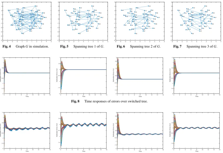
Fig. 4 GraphGin simulation. Fig. 5 Spanning tree 1 ofG. Fig. 6 Spanning tree 2 ofG. Fig. 7 Spanning tree 3 ofG.

Fig. 8 Time responses of errors over switched tree.

Fig. 9 Time responses of errors over sensor network with communication jitters.

algorithms to recalculateLi. The unsteady Kalman filter algorithms need to calculate Riccati differential equation, but do not need the real-time calculation of eigenvalues or an in- verse matrix. Therefore, the assumption that each node has the ability to execute Algorithm 1 is reasonable.

4. Numerical Simulation

Let us consider the quadruple tank system[21]as follows:

A=







−0.15 0 0.5 0

0 −0.25 0 0.5

0 0 −0.15

0 0 0 −0.25





 ,

B= 0.4 0 0 0.4

0 0.4 0.4 0

!T

, u=

cos(πt)+1 sin(πt)+1T

.

There are 50 sensor nodes with the communication paths which are illustrated in Fig. 4. Each sensor in Fig. 4 mea- suresx1 or x2. The topology of the sensor network is gen- erated by a BA model. Letv_i:=(x_gi, y_gi) be a coordinate of nodeiin Fig. 4. We set the observation matrix of each node as

Algorithm 1 Recalculation of ˆCi, ¯Ci j andLiin Each Time Sequence

ifJ_iis modified attthen δ_i(t)←true else

δi(t)←false end if

for alljsuch thatj∈J_ido ifδ¯ji(t−Di j)=truethen

C¯_ji←C¯^new_ji end if end for

for alljsuch thatj∈J_ido δ¯_{i j}(t)←δ_i(t)∨W

k∈J_i\{j}δ¯_ki(t−D_ik) ifδ¯i j(t)=truethen

C¯_{i j}^new←C_i+P

k∈J_i\jC¯_kie⁻^AD^ik end if

end for δˆi(t)←δi(t)∨W

k∈J_iδ¯ki(t−D_jk) ifδˆi(t)=truethen

Cˆ_i←C_i+P

j∈J_iC¯_jie^−AD^{i j}

CalculateLisuch thatA−LiCˆibecomes stable.

end if

Ci=

















0.02 0 0 0

0 0 0 0





, ifxgi>0







0 0 0 0

0 0.02 0 0





, otherwise

. (30)

(8)

i j = kvi−vjk ×0.1.

In a first simulation, the three topologies in Figs. 5, 6 and 7 are switched every 4 seconds. These topologies are the subgraphs of Fig. 4 which have tree structures. Figure 8 shows the time responses of the estimation errors onx1,x2, x3, andx4. After the estimation errors converge to zero, the parameter modifications do not affect the estimates. There- fore, we can confirm that the observer proposed in this paper can estimate the state over the switched tree. In a second simulation, Fig. 5 with communication jitters are used. Let the delays with the jitters be

Dˆi j=(ξ+1)D_{i j},

whereξ∈[0,0.15] is the uniform random number. Figure 9 shows the time responses of the estimation errors onx₁,x₂, x3, and x4 with the communication jitters. The proposed method can estimate the states with a sufficient accuracy over the network with the communication jitters. Therefore, these numerical simulation results verify the effectiveness of the proposed observer and data aggregation method.

5. Conclusion

This paper propose a data-aggregation-based delay compensated observer for a wireless sensor network. The proposed method aggregates the values measured by all the sensors to each node. The communication delay between the neighbor nodes is instantly compensated by each node. Therefore, all of the nodes of a sensor network can estimate the state of the system. The dimensions of the signals on all the communication paths is 2m, which is independent of node number N. This implies that the proposed communication laws are scalable with respect to the network size. A numerical simulation verifies the effectiveness of the proposed method.

In the proposed method, it is assumed that all the nodes can obtain inputs in real time via a fast network. To re- move this assumption, we will consider an observer-based distributed controller in a future study. Moreover, the estimated state of the proposed method and output of the sensor networks have redundancy. We believe that this redundancy could enable us to realize a fault tolerant design for the distributed observers or controllers in wireless networks. This will also be the focus of our future study.

Acknowledgments

This work was partly supported by JSPS KAKENHI Grant Numbers JP16H04380 and JP17K06486.

References

[1] I.F. Akyildiz, W. Su, Y. Sankarasubramaniam, and E. Cayirci, “A survey on sensor networks,” IEEE Commun. Mag., vol.40, no.8, pp.102–114, 2002.

[2] H. Ji, F.L. Lewis, Z. Hou, and D. Mikulski, “Distributed information-weighted Kalman consensus filter for sensor networks,”

Automatica, vol.77, pp.18–30, 2017.

ff

Kalman filtering and smoothing,” IEEE Trans. Autom. Control, vol.55, no.9, pp.2069–2084, 2010.

[4] J. Liang, Z. Wang, and X. Liu, “Distributed state estimation for discrete-time sensor networks with randomly varying nonlineari- ties and missing measurements,” IEEE Trans. Neural Netw., vol.22, no.3, pp.486–496, 2011.

[5] J. Hu, L. Xie, and C. Zhang, “Diffusion Kalman filtering based on covariance intersection,” IEEE Trans. Signal Process., vol.60, no.2, pp.891–902, 2012.

[6] I. Matei and J.S. Baras, “Consensus-based linear distributed filtering,” Automatica, vol.48, no.8, pp.1776–1782, 2012.

[7] G. Battistelli and L. Chisci, “Stability of consensus extended Kalman filter for distributed state estimation,” Automatica, vol.68, pp.169–178, 2016.

[8] V. Ugrinovskii, “Conditions for detectability in distributed consensus-based observer networks,” IEEE Trans. Autom. Control, vol.58, no.10, pp.2659–2664, 2013.

[9] N. Li, S. Sun, and J. Ma, “Multi-sensor distributed fusion filtering for networked systems with different delay and loss rates,” Digit.

Signal Process., vol.34, pp.29–38, 2014.

[10] R. Olfati-Saber, “Distributed Kalman filter with embedded consensus filters,” 44th IEEE Conference on Decision and Control, 2005 and 2005 European Control Conference, pp.8179–8184, IEEE, 2005.

[11] R. Olfati-Saber, “Distributed Kalman filtering for sensor networks,”

46th IEEE Conference on Decision and Control, pp.5492–5498, IEEE, 2007.

[12] R. Olfati-Saber and R.M. Murray, “Consensus problems in networks of agents with switching topology and time-delays,” IEEE Trans.

Autom. Control, vol.49, no.9, pp.1520–1533, 2004.

[13] R. Olfati-Saber and J.S. Shamma, “Consensus filters for sensor networks and distributed sensor fusion,” 44th IEEE Conference on De- cision and Control, 2005 and 2005 European Control Conference., pp.6698–6703, IEEE, 2005.

[14] R.E. Kalman, “A new approach to linear filtering and prediction problems,” J. Fluids Engineering, vol.82, no.1, pp.35–45, 1960.

[15] S. Boyd, A. Ghosh, B. Prabhakar, and D. Shah, “Randomized gossip algorithms,” IEEE Trans. Inf. Theory, vol.52, no.6, pp.2508–2530, 2006.

[16] K. Watanabe and M. Ito, “An observer for linear feedback control laws of multivariable systems with multiple delays in controls and outputs,” Syst. Control Lett., vol.1, no.1, pp.54–59, 1981.

[17] M. Krstic, Delay Compensation for Nonlinear, Adaptive, and PDE Systems, Springer, 2009.

[18] D. Tsubakino, M. Krstic, and T.R. Oliveira, “Exact predictor feed- backs for multi-input LTI systems with distinct input delays,” Auto- matica, vol.71, pp.143–150, 2016.

[19] R. Rajagopalan and P.K. Varshney, “Data aggregation techniques in sensor networks: A survey,” IEEE Commun. Surveys Tuts., vol.8, no.4, pp.48–63, 2006.

[20] T. Tanaka, K.K.K. Kim, P.A. Parrilo, and S.K. Mitter, “Semidef- inite programming approach to Gaussian sequential rate-distortion trade-offs,” IEEE Trans. Autom. Control, vol.62, no.4, pp.1896–

1910, 2017.

[21] K.H. Johansson, “The quadruple-tank process: A multivariable lab- oratory process with an adjustable zero,” IEEE Trans. Control Syst.

Technol., vol.8, no.3, pp.456–465, 2000.

(9)

Ryosuke Adachi received his B.E.

and M.I.S. degrees from Hokkaido University, Japan, in 2014 and 2016, respectively. He is cur- rently a Ph.D. student at the Graduate School of Information Science and Technology, Hokkaido University. His research interests include an estimation of distributed control systems.

Yuh Yamashita received his B.E., M.E., and Ph.D. degrees from Hokkaido University, Japan, in 1984, 1986, and 1993, respectively. In 1988, he joined the faculty of Hokkaido Univer- sity. From 1996 to 2004, he was an Associate Professor at the Nara Institute of Science and Technology, Japan. Since 2004, he has been a Professor of the Graduate School of Information Science and Technology, Hokkaido University.

His research interests include nonlinear control and nonlinear dynamical systems. He is a member of the SICE, ISCIE, RSJ, and IEEE.

Koichi Kobayashi received the B.E. degree in 1998 and the M.E. degree in 2000 from Hosei University, and the D.E. degree in 2007 from To- kyo Institute of Technology. From 2000 to 2004, he worked at Nippon Steel Corporation. From 2007 to 2015, he was an Assistant Professor at Japan Advanced Institute of Science and Tech- nology. Since 2015, he has been an Associate Professor at the Graduate School of Information Science and Technology, Hokkaido University.

His research interests include analysis and control of discrete event and hybrid systems. He is a member of the IEEE, IEEJ, IEICE, and ISCIE.