PAPER
Randomization Approaches for Reducing PAPR with Partial Transmit Sequence and Semidefinite Relaxation
Hirofumi TSUDA†a),Nonmember andKen UMENO††b),Member
SUMMARY To reduce peak-to-average power ratio, we propose a method of choosing suitable vectors in a partial transmit sequence tech- nique. Conventional approaches require that a suitable vector be selected from a large number of candidates. By contrast, our method does not include such a selecting procedure, and instead generates random vectors from the Gaussian distribution whose covariance matrix is a solution of a relaxed problem. The suitable vector is chosen from the random vectors.
This yields lower peak-to-average power ratio than a conventional method.
key words: orthogonal frequency division multiplexing (OFDM), peak-to- average power ratio (PAPR), partial transmit sequence, semidefinite relax- ation, randomization algorithm
1. Introduction
Orthogonal Frequency Division Multiplexing (OFDM) sys- tems are widely used and their signals are generated by Inverse Fast Fourier Transformation (IFFT)[1]. One ad- vantage for OFDM systems is that OFDM systems can deal with multi-path delay since OFDM systems are implemented with IFFT, and effects of multi-path delay in frequency selec- tive channels can be removed with guard interval techniques and zero padding techniques [2]. Since OFDM systems can remove the effects of multi-path delay, Multiple-Input Multiple-Output (MIMO) systems with OFDM systems have been investigated[3].
While there are some advantages in OFDM systems, there are two main problems. One is that signals of OFDM systems have relatively large side-lobes[4]. This problem is caused since OFDM signals consists of sine waves. The other is that signals of OFDM systems have large Peak- to-Average Power Ratio (PAPR), which is the ratio of the maximum value of RF signal powers to the average value of them. Approximately, the output power grows linearly for low values of the input powers. However, for input signals with large power, the growth of the output power is non- linear. Then, in-band distortion and out-of-band distortion are caused for a large input power[5]. With symbols chosen independently, PAPR for OFDM signals has been investi- gated in[6],[7]. Further, in such a case, it has been proven that a baseband-signal can be regarded as a Gaussian process
Manuscript received November 25, 2019.
Manuscript revised July 20, 2020.
Manuscript publicized September 1, 2020.
†The author is with T&S inc., Yokohama-shi, 220-0012 Japan.
††The author is with the Kyoto University, Kyoto-shi, 606-8501 Japan.
a) E-mail: [email protected] b) E-mail: [email protected]
DOI: 10.1587/transfun.2019EBP3243
[8]. With dependent symbols, for example, Bose-Chaudhuri- Hocquenghem (BCH) codes, their PAPR has been investi- gated[9]. Further, the performance of OFDM systems with non-linear amplifiers has been investigated in[10],[11].
To reduce PAPR, many methods have been proposed and explored. For example, a selected mapping method[12], a balancing method[13], an active constellation extension method [14], a tone injection method [15], a complement block coding method[16], a constellation reshaping method [17], an iterative filtering method[18], and a compounding method[19]. These methods are summarized in[20]–[22].
One of the methods to reduce PAPR is a Partial Transmit Sequence (PTS) technique[23]–[26]. PTS techniques are to multiply symbols by phases to reduce PAPR. It is necessary to transmit the vector as side information to the receiver. This yields that OFDM signals are not distorted since we only modulate symbols. Then, their side lobes stay unchanged.
With PTS techniques, there is a significant task for re- ducing PAPR, how to reduce the calculation amount. In[23], a suitable vector is chosen as one which achieves the low- est PAPR from all of the candidates. Then, the calculation amount exponentially gets larger as the length of a vector increases. To reduce such calculations, some methods have been known. In[27], a neighborhood search algorithm has been proposed. With this method, we can obtain a local op- timal solution. Another method is a phase random method [28]. This method consists of generating random vectors whose phase is uniformly distributed in the set of the candi- dates.
In this paper, we propose a method to search the vector which achieves low PAPR. The main point of our method is to obtain the vector from a set of random vectors generated from the Gaussian distribution. Therefore, our method is similar to the phase random method. Then, we derive the optimization problem to reduce PAPR and obtain a solution from the relaxed problem. We regard the solution as a covariance matrix and we can determine the Gaussian distribution.
Our method is a probabilistic scheme since the vectors are generated from a Gaussian distribution. There are some probabilistic schemes in PAPR reduction techniques. A se- lective mapping method was proposed in [12] to generate phases randomly to obtain independent vectors. In[29], for a PTS technique, it has been proposed to choose sub-blocks randomly. Therefore, our method is one such scheme.
The rest of this paper is organized as follows: Section 2 shows the definitions of PAPR and Peak-to-Mean Envelope Power Ratio (PMEPR). In the literature, these two notions Copyright © 2021 The Institute of Electronics, Information and Communication Engineers
sometimes are assumed to coincide, however, these two are different since PAPR and PMEPR are defined with RF sig- nals and base-band signals, respectively. In this section, we clarify the property of signals considered in this paper. Sec- tion 3 shows a partial transmit sequence technique and an optimization problem. It is not straightforward to solve this optimization problem since the feasible region of this opti- mization problem is discrete. Therefore, in Sect. 4, we show a semidefinite relaxation technique to solve it. With this technique, we can obtain approximate solutions. In Sect. 5, we consider random vectors generated from the Gaussian distribution whose covariance matrix is the solution of the relaxed problem. Then, in Sect. 6, we show the relation between our randomization method and the phase random method, which is a conventional method. In Sect. 7, since our problem stated in Sects. 4 and 5 has the large number of constraints, we propose another optimization problem to reduce the upper bound of PAPR. This problem has fewer constraints than the problems in Sects. 4 and 5. Finally, we compare the PAPR of our method with one of existing methods.
The two conference papers by the present authors [25],[26]have shown the randomization methods with cer- tain parameters, which is summarized in this paper. The new contribution of this paper is that more general meth- ods are proposed. We obtain the optimization problem with each kind of parameters and clarify the relation between our methods and the phase random method, which is described in Sect. 6. Further, we consider the upper bound of PAPR and obtain the optimization problem, which is described in Sect. 7. In Sect. 8, we investigate the Bit Error Rate perfor- mances with our methods and existing ones.
2. OFDM System Model and PAPR
In this section, we fix the model and the quantities used throughout this paper. A complex baseband OFDM signal is written as[1]
s(t)= XK
k=1
Akexp 2πjk−1 T t
!
, 0≤t <T, (1)
whereAk is ak-th transmitted symbol,K is the number of symbols,jis the unit imaginary number, andTis a duration of symbols. It is known that OFDM signals are generated by Inverse Fast Fourier Transformation (IFFT)[1]. As seen in Eq. (1), the OFDM signals have no cyclic prefixes. With the cyclic prefix technique, the PAPR is preserved since the cyclic prefix does not induce any new peaks[32]. Therefore, we consider such OFDM signals written in Eq. (1).
A Radio Frequency (RF) OFDM signalζ(t)is written with Eq. (1) as
ζ(t)=Re{s(t)exp(2πj fct)}
=Re
K
X
k=1
Akexp 2πj k−1 T +fc
! t
!
, (2)
where Re{z}is the real part ofz, andfcis a carrier frequency.
With RF signals, PAPR is defined as[30],[31]
PAPR= max
0≤t<T
Re
XK
k=1
Akexp 2πj k−1 T +fc
! t
!
2
Pav ,
(3) wherePavcorresponds to the average power of signals,Pav= PK
k=1E{|Ak|2}, and E{X}is the average ofX. Similarly, with baseband signals, PMEPR is defined as[30],[31]
PMEPR= max
0≤t<T
K
X
k=1
Akexp 2πjk−1 T t
!
2
Pav . (4)
From Eqs. (3) and (4), PAPR and PMEPR are determined if the transmitted symbols{Ak}are given. In the literature, PAPR and PMEPR have often been evaluated as probabil- ities, since PAPR and PMEPR depend on symbols Ak that can be regarded as random variables[6],[9].
Obviously, PAPR does not always correspond to PMEPR. Further, from Eqs. (3) and (4), PAPR does not exceed PMEPR. In [32], under some conditions described below, it has been proven that the following relations are established
1−π2K2 2r2
!
·PMEPR≤PAPR≤PMEPR, (5) whereris an integer such thatfc=r/T. The conditions that Eq. (5) holds areK rand exp(2πj K/r)≈1. In addition to these, another relation has been shown in [21]. Equa- tion (5) implies that PMEPR approximately equals PAPR for sufficiently large fc. It is often the case that PMEPR is evaluated instead of PAPR[6]. In what follows, we assume that the carrier frequency fcis sufficiently large, that is, we consider baseband OFDM signals instead of RF signals.
3. Partial Transmit Sequence Technique
With OFDM systems, the Partial Transmit Sequence (PTS) technique has been proposed to reduce PAPR. In this section, we show the model and the details of PTS techniques. PTS techniques need a vector to reduce PAPR. A disadvantage of PTS techniques is that a large amount of calculation is necessary in some situations. The details of PTS techniques are described in[21],[23],[33].
The symbols in the paper and how to derive index sets for symbols are given as follows. We assume that the sym- bols Ak are given and the number of the symbols is K.
Further, the index set Λ={1,2, . . . ,K}corresponds to the set of unordered symbols{A1,A2, . . . ,AK}. To apply a PTS technique, we divide the index setΛintoPdisjoint subsets, Λ1, . . . ,ΛP, that is,
Λ=Λ1∪ · · · ∪ΛP, Λk∩Λm=∅ if k,m (6)
fork,m=1,2, . . . ,P. There are some discussions about how to divide the index set. We refer the reader to[29],[34],[35].
To express the instantaneous power, we define some quantities as below. For each subsets of symbols, we intro- duce a rotation vectorb = (b1,b2, . . . ,bP)>, where x> is the transpose ofx. The vectorbis chosen as one satisfying bp =exp(jθp)forp=1,2, . . . ,P, whereθp ∈[0,2π). This bplays various roles throughout this paper. For convenience, let us define the quantities
A(p)k =
( Ak k∈Λp
0 otherwise (7)
fork=1,2, . . . ,K andp =1,2, . . . ,P. WithAk(p), a modi- fied baseband OFDM signal ˆs(t)is written as
ˆ s(t)=
P
X
p=1 K
X
k=1
A(p)k bpexp 2πjk−1 T t
!
. (8)
Note that the average power of modified signals is equivalent to one of the original OFDM signals since|bp|=1. With a matrix and vectors, the above equation is rewritten as
ˆ
s(t)=v>t Ab, (9)
where vt=
v1,t v2,t · · · vK,t >
,
A=
* . . . . . . ,
A(1)1 A(2)1 · · · A1(P) A(1)2 A(2)2 · · · A2(P) ... ... . .. ... A(1)K A(2)K · · · AK(P)
+ / / / / / / -
(10)
and
vk,t=exp 2πjk−1 T t
!
. (11)
Note that the matrixAis aK×Pmatrix. With these quan- tities, the instantaneous power|s(t)|ˆ 2is written as
|s(tˆ )|2 =b∗A∗(v∗t)>v>tAb, (12) wherez∗andX∗are the complex conjugate transposes ofz andX, respectively. Here, we have used the fact (v>)∗ = (v∗)>. We denote byCtthe matrixA∗(v∗t)>v>t A. Note that Ctis a positive semidefinite matrix sinceCtis a Gram matrix and each value ofbp is chosen as one achieving the lowest PAPR.
At the receiver side, to recover symbols, it is necessary for the receiver to know the explicit values ofb. Note that Signal to Noise Ratio (SNR) is preserved if the receiver knows b. To let the receiver know, the vector b has to be transmitted as side-information. To reduce information content, the value ofbp is usually restricted to
bp ∈ (
1,exp 2πj1 L
!
, . . . ,exp 2πjL−1 L
! )
, (13)
where L is a positive integer. We denote by ΩL the set (1,exp
2πjL1
, . . . ,exp
2πjL−1L )
. From the above defi- nition, the vector bbelongsΩPL, whereΩPL is a P-tuple of ΩL. Then, the information content of b is (P−1)log2L [bits] since we can setb1 =1 without loss of generality. It is obvious that the number of elements in the setΩP−1
L isLP−1. Letb?be the optimal vector which achieves the lowest PAPR inΩPL. Then, it turns out thatb?is the global solution of the optimization problem
(QL) min max
0≤t<T|s(t)|ˆ 2
subject to bp ∈ΩL (p=1,2, . . . ,P). (14) Our aim is to find the vectorb?. To this end, there are two main obstacles to solve the problem(QL).
One obstacle is that the timet is continuous. In[32], with baseband OFDM signalss(t)defined in Eq. (1), it has been shown that there is the following relation between con- tinuous signals and sampled signals
0max≤t<T|s(t)| <
s J2
J2−π2/2 max
0≤n<J K
s nT J K
!
, (15)
where Jis an integer satisfying J > π/√
2. Equation (15) implies that PMEPR can be estimated precisely from signals sampled with a sufficiently large oversampling factor. For maxima of continuous signals and sampled signals, other relations have been shown in [36], [37]. The integer J is often called a oversampling factor[10], and is often chosen asJ≥4. How to choose the oversampling factorJhas been discussed in[32].
With sampled signals, the problem(QL)is rewritten as (QˆL) minλ
subject to b∗CnT/(J K)b≤λ (n=0,1, . . . ,J K−1) λ∈R, bp ∈ΩL (p=1,2, . . . ,P).
(16) Note that the variables in the problem(QˆL)arebandλ.
The other obstacle is that the feasible region ΩL is discrete. In[23], a brute-force search has been used to find the global solutionb?. With this method, we have to find the vector b? from LP−1 candidates, and the calculation amount exponentially gets larger asPincreases. In[27], the neighborhood search algorithm has been proposed. With this method, we can obtain a local optimal solution. However, it is only known that its calculation amount is proportional to
P−1Cr ·Lr, wherer is an integer parameter expressing the distance of a neighborhood andaCbis a binomial coefficient.
Another existing method is the phase random method[28].
This method consists of generating random vectors whose phase is uniformly distributed in the regionΩPL, from which we obtain a solution.
4. Semidefinite Relaxation
Since it is not straightforward to obtain the global solu-
tion, we propose an efficient method to obtain a solution which achieves low PAPR. Optimization problems, such as the problem(QˆL), appear in MIMO detection[38]. Thus, we can use these methods that have already been developed to our problem. One of such existing methods uses a semidef- inite relaxation technique[39]. In this section, we obtain a solution with such semidefinite relaxation techniques.
We apply semidefinite relaxation techniques to the prob- lem(QˆL). Our main aim is to change the variablebto a pos- itive semidefinite matrixX. The ways to solve the problem (QˆL)depend onΩL. Therefore, we consider each problem for various cases ofL.
4.1 Optimization Problem forL=2
First, we consider the problem(QˆL)forL=2,(Qˆ2). Then, Ω2 ={−1,1}. Note thatb2 =1 forb∈Ω2. If we define the matrix X = bb>, then X is a positive semidefinite matrix whose rank is 1 and the problem(Qˆ2)is rewritten as
(Qˆ2) minλ
subject to Tr(CnT/(J K)X)≤λ (n=0,1, . . . ,J K−1) rank(X)=1, Xp,p=1 (p=1,2, . . . ,P) X <0, X ∈SP, λ∈R,
(17) where Tr(X) is the trace of X, rank(X) is the rank of X, X <0 indicates thatXis a positive semidefinite matrix and SPis the set of symmetric matrices of dimensionP. Due to the constraint rank(X)=1, the problem(Qˆ2)is not convex.
Note that the set of positive semidefinite matrices is convex [40]. By dropping the rank constraint, we obtain the relaxed optimization problem
(Qˆ20) minλ
subject to Tr(CnT/(J K)X)≤λ (n=0,1, . . . ,J K−1) Xp,p =1 (p=1,2, . . . ,P)
X <0, X ∈SP, λ∈R.
(18) The above problem (Qˆ02) can be solved since the problem (Qˆ02)is convex. LetX2?be the global solution of the problem (Qˆ02). If the rank of X2? is 1, then we obtain the global solution of the problem(Qˆ2), denoted byb?2. However, the rank ofX?2 is not always 1. To deal with this, we obtain an approximate solution fromX2?as follows. First, the solution X2?is decomposed as
X2?=
r2
X
i=1
λiqiq∗i, (19)
wherer2 = rank(X2?), λi is the eigenvalue of X2?, λ1 ≥ λ2 ≥. . . ≥ λr2 andqi is the respective eigenvector. Then, in a least-two-norm sense, the approximate solution whose rank 1 is obtained as ˆX2?=λ1q1q∗1. From this approximate
solution, we systematically obtain the solution of the original problem(Qˆ2)as√
λ1q1. However, this solution is not always in the feasible region of the problem (Qˆ2). To have an approximate solution in the feasible region, for the problem (Qˆ2), we need to project the solution onto the feasible region.
We finally arrive at the p-th element of the approximate solution of the problem(Qˆ2)as
bˆ2,p=sgn(q1,p), (20)
whereq1,pis thep-th element ofq1and sgn(x)=
( 1 x≥0
−1 x<0 . (21)
We call this technique “l2approximation method”.
4.2 Optimization Problem forL=4
Similar to the caseL=2, we obtain the approximate solution of the problem (Qˆ4). For L = 4, the setΩ4 is written as Ω4={1,exp(jπ/2),−1,exp(j3π/4)}. To obtain the relaxed problem, we rewrite the problem(Qˆ4)as follows. First, let us define the set
Ωˆ4 ={+1+j,+1−j,−1+j,−1−j}, (22) which can be expressed as
Ωˆ4 ={
√
2 exp(jπ/4)·a|a ∈Ω4}. (23) Note that Re{b}2 = Im{b}2 = 1 for b ∈ Ωˆ4 and that the elements in ˆΩ4 are complex. Second, we rewrite the set ˆΩ4 in terms of real parts and imaginary parts. To this end, we introduce the following transformations forz∈CnandZ ∈ Hn, whereHnis the set of Hermitian matrices of dimension n[41],
T(z)= Re{z}
Im{z}
!
, and T(Z)= Re{Z} −Im{Z}
Im{Z} Re{Z}
! . Note thatT(X)∈S2nifX ∈Hn[42]. Finally, we arrive at the relaxed problem forL=4.
(Qˆ04) minλ
subject to Tr(CˆnT/(J K)X)≤λ (n=0,1, . . . ,J K−1) Xp,p=1 (p=1,2, . . . ,2P)
X <0, X ∈S2P, λ∈R,
(24) where ˆCt=T(Ct). Note that the problem(Qˆ04)is equivalent to (Qˆ4) if we impose the rank constraints to the problem (Qˆ40)and the problem(Qˆ04)is convex. LetX4?be the global solution of the problem (Qˆ04). From X4?, we can obtain an approximate solution by the following procedure. First, we decomposeX?4 as
X4?=
r4
X
i=1
λiqiq∗i, (25)
wherer4 =rank(X4?),λiis the eigenvalue ofX?4,λ1≥λ2≥ . . . ≥ λr4, andqi is the respective eigenvector. From the vectorq1, we can obtain the approximate solution ˆb4 ∈CP written as
bˆ4,p= 1
√
2exp(−jπ/4)
sgn(qp)+j·sgn(qp+P) ,
(26) where ˆb4,p andqp are thep-th elements of ˆb4 andq1, re- spectively.
4.3 Optimization Problem for GeneralL For generalL, we consider the relaxed problem
(Qˆ0L) minλ
subject to Tr(CnT/(J K)X)≤λ (n=0,1, . . . ,J K−1) Xp,p =1 (p=1,2, . . . ,P)
X <0, X ∈HP, λ ∈R.
(27) Note that the set of Hermitian positive semidefinite matrices is convex[39]and the above problem(Qˆ0L)is convex. The problem (Qˆ0L) is not equivalent to the problem (QˆL) for L , 2,4 if the rank constraint is imposed. Similar to the problem forL =2 andL =4, letX?Lbe the global solution of the problem(Qˆ0L). Then,X?Lis decomposed as
X?L=
rL
X
i=1
λiqiq∗i, (28)
whererL=rank(X?L),λiis the eigenvalue ofXL?,λ1≥λ2≥ . . . ≥ λrL andqi is the respective eigenvector. From the vectorq1, we can obtain the approximate solution ˆbL ∈CP as
bˆL=arg min
b∈ΩPL
kq−bk, (29)
whereq=√
λ1q1andkzkis the Euclidean norm ofz.
5. Randomization Method
In Sect. 4, we have discussed the relaxed problems and how to obtain the approximate solutions. However, clearly, ap- proximate solutions are not suitable if the global solutions of the relaxed problems have some large eigenvalues, that is, the ranks of solutions are not regarded as unity.
In this section, we introduce a randomization method.
This method has been used to analyze how far the optimal value of relaxed problems is from one of original problems [43]. With this method, we obtain solutions as random values which are generated from a Gaussian distribution. Similar to discussions in Sect. 4, we consider each problem for various cases ofL. Further, in the end of this section, we discuss the computational complexity of our randomization method.
5.1 Randomization forL=2
First, we consider the problem forL=2. Letξbe a random vector generated from the Gaussian distribution N(0,X) with zero mean and a covariance matrix X. The definition and properties of a Gaussian distribution have been shown in[44].
To find an approximate solution, we rewrite the problem (Qˆ20)as follows. With
E{ξ>Ctξ}=Tr(CtX), (30) the problem(Qˆ02)can be written as
(Qˆ20) minλ
subject to E{ξ>CnT/(J K)ξ} ≤λ (n=0,1, . . . ,J K−1) Xp,p =1 (p=1,2, . . . ,P)
X <0, X ∈SP, λ∈R, ξ ∼ N(0,X).
(31) Note that the variables of the above problem are X and λ. Then, it is clear that the optimal matrix X?2 defined in Sect. 4 is the optimal matrix of the above problem in a sense of a covariance matrix. This result suggests that a suitable solution can be obtained from a set of random vectors generated from the Gaussian distributionN(0,X2?) [45]. We can then obtain the approximate solution as follows.
1. Solve the problem(Qˆ20)and obtain the covariance ma- trixX2?.
2. Generate random vectors {ξ} from the Gaussian dis- tributionN(0,X2?) and project them onto the feasible region of the original problem(QˆL), that is, forL=2, obtain the projected solutions
bˆp =sgn ξp
(p=1,2, . . . ,P), (32) whereξpis thep-th element ofξ.
3. Choose the solution which achieves the minimum PAPR among all the random vectors and regard it as an ap- proximate solution.
5.2 Randomization forL=4
Similar to the case for L =2, we can obtain the covariance matrixX4?forL=4 and obtain random vectors{ξ}generated fromN(0,X4?). Since the dimension of the vectors{ξ}is 2P, the projected one is written as
bˆp = 1
√
2exp(−jπ/4)
sgn(ξp)+j·sgn(ξp+P) (33) forp =1,2, . . . ,P. From these random vectors, we choose an approximate solution which achieves the minimum PAPR among them.
5.3 Randomization with GeneralL
For generalL, we can obtain the complex covariance matrix X?Las a solution of the problem(Qˆ0L). Similar to the meth- ods forL=2 andL=4, our goal is to choose the solution from random vectors. The main part of our method is to ob- tain an approximate solution from random vectors generated from the complex Gaussian distribution CN(0,XL?). The definition and the detail of a complex Gaussian distribution have been shown in[46]. There have been some methods to obtain an approximate solution from random vectors[47]–
[49], and our method is a special case of an algorithm in [49]. From the complex Gaussian distributionCN(0,XL?), we can obtain the random vectors {ξ}. Then, we have to transform the random vectors{ξ}into feasible ones as so- lutions of the problem(QˆL). Our transformation method is written as follows. Let fLbe
fL(z)=
1 Argz∈[0,L12π) ...
ωlL Argz∈[Ll2π,l+1L 2π) ...
ωL−1L Argz∈[L−1L 2π,2π)
, (34)
wherez∈C,ωL =exp(2πj/L)and Argzis the angle ofz.
With the functionfL, the random vectorξgenerated from the complex Gaussian distributionCN(0,X?L)is transformed to bˆp= fL(ξp) (p=1,2, . . . ,P). (35) It is clear that ˆbp ∈ΩL. Therefore, ˆbis a feasible solution of the problem(QˆL). With the above method, we can obtain the feasible solutions from random vectors generated from the complex Gaussian distribution CN(0,X?L). Then, we choose the approximate solution from them which achieves the minimum PAPR among the set of the random vectors.
Our method is summarized in Algorithm 1.
Algorithm 1:Randomization Method with Semidef- inite Relaxation
1 Obtain the relaxed problem with semidefinite relaxation techniques.
2 Obtain the positive semidefinite matrixX?as the optimal solution of the relaxed problem.
3 Determine the Gaussian distributionN(0,X?)(withL,2,4, C N(0,X?)is determined). Then, generateNsamples from the Gaussian distribution as the candidates of the solution.
4 Project the samples onto the feasible region, and obtain the projected samples.
5 Choose the solutionb?from the projected samples which achieves the minimum PAPR. Then, outputb?as the solution.
5.4 Computational Complexity
There are many discussions about computational complexi- ties of PAPR reduction techniques. In this section, we discuss
the computational complexity of our randomization method under the condition that the disjoint index subsets Λp are given. The remaining complexities consists of three parts:
(i) to generate random vectors, (ii) to choose the optimal vec- tor from the random vectors, and (iii) to obtain the solution of the optimization problem.
In generating random vectors, computational complex- ity is in proportion to the number of random vectors. The computational complexity turns out to beN·cgen, whereN andcgenare the number of random vectors and the computa- tional cost for generating each random vector, respectively.
Similarly, in choosing the optimal vector from given random vectors, its computational complexity isN·J K·ccal, where ccalis the computational cost for calculating the amplitude of each samples,JandK have been defined in Sects. 3 and 2, respectively.
When we solve the optimization problem to obtain the solution, the computational complexity for solving the opti- mization problem is not clear since our optimization problem is not an ordinary semidefinite relaxation problem written in [39]. In this paper, we assume that the computational com- plexity of our optimization problem is nearly equivalent to one of ordinary semidefinite relaxation problems. Then, the worst case complexity is O(max{m,n}4n1/2log(1/)), whereOrepresents the order,mis the number of constraints, nis the dimension of the matrix, and >0 is solution accu- racy[39]. For the generalL, since the optimization problem (Qˆ0L)has(J K+P)constraints, the worst case complexity is O((J K+P)4P1/2log(1/)).
6. Relation between Our Method and Phase Random Method
In Sect. 5, we have shown our randomization method. Sim- ilar to our method, the phase random method has been pro- posed[28]. This method uses random vectors whose phase is uniformly distributed inΩL. In this section, we discuss the relation between our method and the phase random method.
First, we explain the phase random method. We define the probability mass function as
Pr( z=ωlL)
= 1
L (l=0,1, . . . ,L−1), (36) whereωL =exp(2πj/L), which has been defined in Sect. 5.
Thus, ωL ∈ ΩL and phases are uniformly distributed in ΩL. With this probability, the phase random method is summarized in Algorithm 2.
Algorithm 2:Phase Random Method
1 Let the number of the samples beN. Generate the variable zn,p ∈ΩLwith the probability Pr(
z=ωlL) for n=1,2, . . .,Nandp=1,2, . . .,P−1.
2 Obtain the set of vectors{z}as zn=(1,zn,1,zn,2, . . .,zn,P−1)>.
3 Choose the vectorz?which achieves the lowest PAPR from{z}.
Further, let us discuss the complex Gaussian distribu- tion. From [46], if z ∈ Cn follows CN(µ,Σ), then the probability density function ofT(z) ∈R2nis the Gaussian distributionN
T(µ),12T(Σ)
. Therefore, we can consider a real-value Gaussian distribution instead of a complex Gaus- sian distribution.
Let us consider the complex Gaussian distribution CN(0,IP), whereIPis the identity matrix whose size isP.
It is clear that the matrixT(IP)is the identity matrix whose size is 2P. From the above discussion, and the covariance matrix is identity matrix, each variable ofzgenerated from CN(0,IP)is uncorrelated. It is known in[50]that uncorre- latedness is equivalent to independence for normal variables.
Therefore, it is sufficient to consider a vectorzwhose ele- ment is generated from the complex Gaussian distribution CN(0,1). The variablezwhich is the element ofzcan be decomposed asz=x+jy,wherexandyare real numbers following the independent Gaussian distributionN(0,1/2), respectively.
Let us definer ≥0 andθ ∈ [0,2π) so thatx+jy = rexp(jθ). Then, sincexandyare normal variables follow- ingN(0,1/2), the probability density ofθ∈[0,2π)is
p(θ)= 1
2π, (37)
from which, the phase of a variable z generated from CN(0,1)is uniformly distributed[50].
From the above discussions and the definition of the function fL(z), the probability mass function of fL(z) is written as
Pr(
fL(z)=ωlL)
= 1
L. (38)
This result implies that the phase random method is equiv- alent to our method whose covariance matrix is the identity matrix with the function fL(z).
7. Reducing Upper Bound of PAPR
We have discussed how to obtain a covariance matrix to de- termine a Gaussian distribution. In Sect. 5, we have obtained the optimization problem(Qˆ0L). This problem contains the oversampling parameter J. As seen in Sect. 3, measured PAPR calculated from sampled signals converges to the true value of PAPR as J → ∞. Therefore, a sufficiently large Jis necessary to evaluate PAPR tightly. Then, however, as seen in Sect. 5, the number of constraints in the optimization problem(Qˆ0L)gets larger asJincreases. In such a situation, the optimization problem(Qˆ0L)gets complicated.
To overcome this obstacle, instead of PAPR, we con- sider an optimization problem to reduce the upper bound of PAPR which does not depend on timet. From this problem, we obtain a covariance matrix as the solution.
In this section, we consider a generalL. Then, specify- ingL=2,4, we can verify the same results for ones obtained in this section with the techniques discussed in Sect. 4 as fol- lows. With L = 2, the set of matrices is the symmetric
matricesSP, and withL=4, we replace a positive semidef- inite matrixXwithT(X).
The upper bound of the signal envelope has been shown with Eq. (1) as[51]
|s(t)|2 ≤
K
X
k=1
|Ak|2+2
K−1
X
i=1
|ρ(i)|, (39)
where ρ(i)=
K−i
X
k=1
AkAk+i (40)
andzis the complex conjugate ofz. We letρ(K)=0 for lat- ter convenience. The right hand side of Eq. (39) is indepen- dent of the timet. Let us defineρ0=(ρ(1), ρ(2), . . . , ρ(K− 1))>. Note that the first term in right side of Eq. (39), PK
k=1|Ak|2, corresponds to ρ(0) and this term is not var- ied with PTS techniques since each element of a vector bn satisfies|bn|=1.
From the above discussion, without taking into account convexity, it is expected to decrease PAPR when we re- duce kρ0kl1, where kzkl1 is the l1-norm of z. However, it is not the case since each |ρ(i)| is not convex if we re- gard Ak as variables. Therefore, we use l2-norm of ρ0, kρ0kl2. From the Cauchy-Schwarz inequality, it follows that kρ0kl1 ≤
√
K−1kρ0kl2. Therefore, kρ0kl1 is expected to decrease whenkρ0kl2 decreases.
Let us consider the following vector ρˆ =(ρ(0),√
2ρ(1), . . . ,√
2ρ(K−1))>. (41) It is clear that minimizingkρˆkl2is equivalent to minimizing k
√2ρ0kl2sinceρ(0)is constant. Then,kρˆk2
l2is written as kρkˆ l2
2=2
K−1X
k=1
|ρ(k)|2+|ρ(0)|2
=
K−1
X
k=0
|ρ(k)|2+
K−1
X
k=0
|ρ(K−k)|2
=1 2
K−1X
k=0
|ρ(k)+ρ(K−k))|2+|ρ(k)−ρ(K−k)|2
. (42) Here,ρ(k)denotes the complex conjugate ofρ(k). From the above equations,kρˆk2
l2is divided into a periodic correlation term and an odd periodic correlation term. With Eq. (8), these terms are written as
ρ(k)+ρ(K−k)=b∗A∗B1,1(k)Ab,
ρ(k)−ρ(K−k)=b∗A∗B−1,1(k) Ab, (43) where the matricesB1,1(k)andB−1,1(k) are written as
B1,1(k)= O Ik
IK−k O
!
, B−1,1(k) = O −Ik
IK−k O
! .
(44)
Since these matrices are regular, they can be transformed to diagonal matrices. With this general discussion, these matrices are decomposed as[52]
B1,1(k)=V∗D(k)V,B−1,1(k) =Vˆ∗Dˆ(k)V,ˆ (45) whereVand ˆVare unitary matrices whose(m,n)-th elements are
Vm,n= 1
√ Kexp
−2πjmn K
, Vˆm,n= 1
√
Kexp −2πjn m K + 1
2K
! ! ,
(46)
andD(k)and ˆD(k)are diagonal matrices whosen-th diagonal elements are
D(kn)=exp
−2πj k n K
, Dˆn(k)=exp −2πj k n K + 1
2K
! ! . (47) With these expressions, Eq. (42) is written as
kρkˆ l2
2 = K
2
K
X
k=1
|αk|4+
K
X
k=1
|βk|4
, (48)
whereαkandβk are thek-th element ofαandβwritten as α =V Abandβ=V Ab, respectively. With the variableˆ b, the above equation is written as
kρkˆ l2
2= K
2
K
X
k=1
b∗A∗V∗GkV Ab2+
b∗A∗Vˆ∗GkV Abˆ 2 , (49) whereGkis a matrix whose(k,k)-th element is unity and the other elements are zero. Note thatGk =G∗kGk. Then, the matricesA∗V∗GkV AandA∗Vˆ∗GkV Aˆ are positive semidef- inite matrices since they are the Gram matrices. Further, Eq. (49) is convex with respect to the variableb. This is proven in Appendix A. From the above discussions, it fol- lows that the squared l2-norm of ˆρ is a convex function with respect to the variableb. Combining these discussions above, we obtain the optimization problem,
(Ql2) minF(b)
subject to bp ∈ΩL (p=1,2, . . . ,P), (50) where
F(b)=
K
X
k=1
b∗A∗V∗GkV Ab2+
b∗A∗Vˆ∗GkV Abˆ 2 . (51) To overcome the obstacle caused by the discreteness ofΩL, we obtain a relaxed problem with semidefinite relaxation techniques. This convex problem is written as
(Q0l
2) min ˆF(X)
subject to Xp,p =1 (p=1,2, . . . ,P) X <0, X ∈HP,
(52)
where F(X)ˆ =
K
X
k=1
A∗V∗GkV AX2+
A∗Vˆ∗GkV AXˆ 2 . (53) From the above discussions, how to obtain the optimal solution as a positive semidefinite matrix has been shown.
Then, we discuss the relations between our randomization method and the relaxed problem (Q0l
2). LetX?and{ξ}be the global solution of the problem(Q0l
2)and the random vec- tors generated from the Gaussian distribution CN(0,X?), respectively. They satisfy E{ξξ∗} = X?. Then, it follows that
K
X
k=1
Tr
A∗V∗GkV AX?2
+Tr
A∗Vˆ∗GkV AXˆ ?2
≤
K
X
k=1
E
ξ∗A∗V∗GkV Aξ2+
ξ∗A∗Vˆ∗GkV Aξˆ 2
≤3
K
X
k=1
Tr
A∗V∗GkV AX?2
+Tr
A∗Vˆ∗GkV AXˆ ?2 . (54) The above relations are proven in Appendix B. Our main aim is to find Xl?
2 minimizing E{F(ξ)} under the constraints, where ξ ∼ CN(0,Xl?
2). Two inequalities are involved in Eq. (54). The first inequality in Eq. (54) implies that the global solution of the relaxed problem X? does not al- ways correspond to Xl?
2. However, the last inequality in Eq. (54) implies thatX?will be an appropriate solution for our randomization method since X? will make E{F(ξ)}
small where ξ ∼ CN(0,X?). From the above discussions, the global solution of the relaxed problem X? is not the optimal covariance matrix with our randomization method minimizing upper bound of PAPR. However,X?will achieve low PAPR with our randomization method.
8. Numerical Results
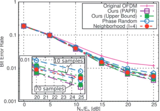
In this section, from the perspective of PAPR and Bit Error Rate (BER), we compare the performances of our random- ization methods with ones of the phase random method and the neighborhood method[27].
Here, we randomly generate transmitted symbols{Ak}. In practical situations, an error correction code is used and transmitted symbols depend on the code. However, it is known that most good codes do not introduce correlation into the symbol stream[8]. This yields that the transmitted symbols are also uncorrelated. Further, as mentioned in [8], a symbol stream is only locally dependent for traditional
codes. Thus, the following numerical results shown in this section will be extended to the case where an error correction code is used.
We numerically solve the problems(Qˆ0L)and(Q0l
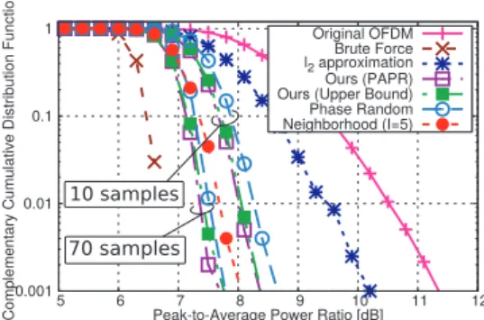
2)with CVX[53] and obtain approximate solutions with the two kinds of methods, thel2 approximation method discussed in Sect. 4 and a random method discussed in Sects. 5 and 7, respectively. As the parameters, the number of carriers K =256 and the oversampling parameter J =16 are cho- sen. We obtain PAPR curves with three kinds of parameters, (P,L)=(16,2),(8,4)and(8,8). The oversampling param- eterJis also used in calculating PAPR (see Eq. (15)). As the modulation scheme, each symbol is independently chosen from 16-QAM symbols. The index sets Λn are randomly chosen from the set{1,2, . . . ,K}and they satisfy|Λn|= KP forn=1,2, . . .P, where|Λn|is the number of components in the setΛn. It has been known that PAPR with random index sets is lower than one with adjacent index sets[29].
With our randomization methods discussed in Sects. 5 and 7, and the phase random method, we generate 10 and 70 sam- ples as solution candidates and choose the optimal solution from such candidates (see Algorithm 1). For the brute force method and the other methods, we draw the PAPR curves from 200 results and 2000 results, respectively. Note that the PAPR curve with the brute force method is optimal. For the neighborhood method, we set the Hamming weight pa- rameterr=1 and the maximum iteration parameterI=5,4 and 3 in(P,L)=(16,2),(8,4)and(8,8), respectively. Note that the number of candidates in the neighborhood method is roughly calculated asI(P−1)(L−1)whenr =1. With these parameters, the number of candidates in the neighbor- hood method is roughly calculated as 70. Thus, the search complexity of the neighborhood method is nearly equivalent to one of our methods.
Figures 1, 2 and 3 show each PAPR curve with orig- inal OFDM systems, the brute force method [23], the l2 approximation method discussed in Sect. 4, the randomiza- tion method discussed in Sect. 5, the reducing-upper bound method discussed in Sect. 7, the phase random method[28]
and the neighborhood method[27]. In the legends, “l2ap- proximation”, “Ours (PAPR)”, “Ours (Upper Bound)” and
“Neighborhood” mean thel2approximation method, the ran- domization method discussed in Sect. 5, the reducing-upper bound method discussed in Sect. 7 and the neighborhood method, respectively. In Fig. 3, the PAPR curve with the brute force method is not drawn since it is not straightfor- ward to obtain the optimal vector due to its significantly large calculation amount. From these figures, the PAPR curve with thel2approximation method is far from one with the brute force method. This result shows that the optimal solution of the relaxed problem is far from a rank-1 matrix and it tends to have some large eigenvalues. Therefore, we conclude that thel2approximation method is not suitable for PTS techniques.
With randomization methods, there are two PAPR curves obtained from 10 random vectors and 70 random vectors. In both numbers of random vectors, the PAPRs
Fig. 1 PAPR with the 16-QAM modulation scheme in the parameters (P,L)=(16,2),K=256 andJ=16.
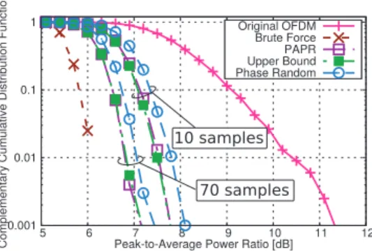
Fig. 2 PAPR with the 16-QAM modulation scheme in the parameters (P,L)=(8,4),K=256 andJ=16.
Fig. 3 PAPR with the 16-QAM modulation scheme in the parameters (P,L)=(8,8),K=256 andJ=16.
of our two randomization methods are lower than those of phase random techniques. As seen in Sect. 6, the phase ran- dom method is equivalent to our method with the identical matrix as a covariance matrix. Therefore, the performance of randomization methods can be improved when a suitable covariance matrix is chosen. Further, with 70 samples, PA- PRs of our two randomization methods are lower than one of the neighborhood method. Since the search region of the neighborhood method is roughly equivalent to ones of our methods, these results show that our methods can find a suit- able vector more efficiently than the neighborhood method.
In Sect. 5, we have discussed the computational com- plexity of our method. Tables 1, 2 and 3 show the aver- aged calculation time for obtaining a solution in our meth-
Table 1 Averaged calculation time for algorithms with the parameters(P,L)=(16,2),J=16 and the 16-QAM modulation scheme.
Ours(PAPR) Ours(Upper Bound) Phase Random 10 iterations 30.79111 [sec] 5.442301 [sec] 0.3556757 [sec]
70 iterations 33.80662 [sec] 6.900336 [sec] 2.458494 [sec]
Table 2 Averaged calculation time for algorithms with the parameters(P,L)=(8,4),J=16 and the 16-QAM modulation scheme.
Ours(PAPR) Ours(Upper Bound) Phase Random 10 iterations 32.78214 [sec] 5.167035 [sec] 0.291365 [sec]
70 iterations 32.86061 [sec] 6.119004 [sec] 2.04702 [sec]
Table 3 Averaged calculation time for algorithms with the parameters(P,L)=(8,8),J=16 and the 16-QAM modulation scheme.
Ours(PAPR) Ours(Upper Bound) Phase Random 10 iterations 20.40021 [sec] 4.669453 [sec] 0.2870807 [sec]
70 iterations 22.47077 [sec] 6.416054 [sec] 2.060964 [sec]
Table 4 Averaged calculation time for the algorithms in the parameters(P,L) =(16,2)and the 16-QAM modulation scheme.
J=4 J=8 J=16
10 iterations 6.513275 [sec] 13.62168 [sec] 30.79111 [sec]
70 iterations 8.060944 [sec] 15.30768 [sec] 33.80662 [sec]
ods and the phase random method with the parameters (P,L) = (16,2),(8,4) and (8,8), respectively. In these parameters, the averaged calculation time of the algorithm proposed in Sect. 5 and the reducing-upper bound method is larger than one of the phase random method. Since an opti- mization has to be solved to obtain a solution in our proposed method, the calculation time of our methods is larger than one of the phase random method. In our methods, the calcu- lation time of the reducing-upper bound method is smaller than one of the method proposed in Sect. 5. The reason may be explained as follows. As seen in Sect. 5, it is expected that the computational complexity depends on the number of constraints which is written in terms ofJ. In the method proposed in Sect. 5, the over sampling parameter J =16 is chosen here. Thus, the number of constraints of the method proposed in Sect. 5 is J K+P = 16K +P. On the other hand, the number of constraints in the reducing-upper bound method is regarded as 2Ksince the objective function of this method consists of 2K terms. Thus, the calculation time of the reducing-upper bound method is smaller than one of the method proposed in Sect. 5 since the number of the con- straints in the reducing-upper bound method is smaller than one of the method proposed in Sect. 5. Thus, these results imply that the large number of constraints implies the large calculation complexity.
We have seen the calculation time for obtaining a solu- tion withJ=16. From the above discussion, it is expected that the calculation time gets smaller as the parameterJgets smaller since the computational complexity will depend on J. Table 4 shows the averaged calculation time for obtaining a solution with severalJin the parameters(P,L)=(16,2).
Here, when we choose the solution from the candidate set,
we use the parameterJ=16 to calculate PAPR. Thus, only the parameter J in the optimization problem is varied. As seen in Table 4, the averaged calculation time gets larger as J gets larger. Note that the oversampling parameter J in the reducing-upper bound method is regarded as J =2.
This yields that the computational complexity gets larger as the parameter J gets larger. Figure 4 shows PAPR curves with several Jfor the parameters(P,L)=(16,2). As seen in this figure, PAPRs of the methods proposed in Sect. 5 with J =4,8 and 16 are lower than one of the phase ran- dom method. From the above discussions, we conclude that the method proposed in Sect. 5 will be efficient with any J.
Note that the parameter Jsatisfies the condition defined in Eq. (15).
In the method proposed in Sect. 5, we have considered the three cases: (i)L =2, (ii)L =4, and (iii) general L. It is clear that the method for generalL can be applied when L=2 orL=4. Here, we verify the efficiency of our method for a general Lin such cases. Figures 5 and 6 show PAPR curves with the algorithm for a general L. In the legend,
“PAPR” and “Upper Bound” denote the method proposed in Sect. 5 and the reducing-upper bound method, respectively.
To draw these two figures, the parameters are chosen as (P,L) = (16,2) and (P,L) = (8,4), respectively. Here, the number of carriers and the parameter J are K = 256 and J =16. These figures show that PAPR of the method proposed in Sect. 5 for a general Lis lower than one of the phase random method. Thus, even in casesL=2 andL=4, our method for a generalLis efficient.
We have seen PAPRs obtained with our methods and some existing methods. These results have been obtained with the 16-QAM modulation scheme and the number of
Fig. 4 PAPRs with someJin the parameters(P,L)=(16,2),K=256 and the 16-QAM modulation scheme.
Fig. 5 PAPR with the generalL-randomization algorithm in the param- eters(P,L) =(16,2),K =256,J =16 and the 16-QAM modulation scheme.
Fig. 6 PAPR with the generalL-randomization algorithm in the param- eters(P,L) =(8,4), K =256,J =16 and the 16-QAM modulation scheme.
carriers K =256. Here, we show some results with other situations. Figure 7 shows PAPR curves withK=128 for the parameters(P,L) = (16,2). Here, the modulation scheme is the 16-QAM. Similar to the results inK=256, PAPRs of our methods are lower than one of the phase random method.
Thus, our methods will be efficient for anyK. Figures 8 and 9 show PAPR curves for the parameters(P,L)=(16,2)and K = 256 in the QPSK modulation scheme and 64-QAM modulation scheme, respectively. Similar to the results in the 16-QAM modulation scheme, our methods can achieve lower PAPRs than the phase random method in the both schemes. From the above discussions, we conclude that our
Fig. 7 PAPR with the 16-QAM modulation scheme in the parameters (P,L)=(16,2),K=128 andJ=16.
Fig. 8 PAPR with the QPSK modulation in the parameters(P,L) = (16,2),K=256 andJ=16.
Fig. 9 PAPR with the 64-QAM modulation in the parameters(P,L)= (16,2),K=256 andJ=16.
method will be efficient with any number of carriers and any modulation scheme.
To explore the performances with our method and the phase random method, we evaluate each BER. To this end, the amplifier model is chosen as the Rapp model[54], which is described below. Let the input signal be presented in polar coordinates,
x(t)=ρ(t)exp(jθ(t)). (55)
Then, the output signal is written as
ζ(x(t))=γ(ρ(t))·exp(j·(θ(t)+Φ(ρ(t)))), (56) whereγandΦare functions of the amplitude ρ(t). In the