Domain Adaptation Based on Mixture of Latent Words Language Models for Automatic Speech Recognition

(1)

PAPER

Domain Adaptation Based on Mixture of Latent Words Language Models for Automatic Speech Recognition

Ryo MASUMURA^†a), Taichi ASAMI^†, Takanobu OBA^†∗, Hirokazu MASATAKI^†, Sumitaka SAKAUCHI^†, andAkinori ITO^††,Members

SUMMARY This paper proposes a novel domain adaptation method that can utilize out-of-domain text resources and partially domain matched text resources in language modeling. A major problem in domain adaptation is that it is hard to obtain adequate adaptation eﬀects from out-of- domain text resources. To tackle the problem, our idea is to carry out model merger in a latent variable space created from latent words language models (LWLMs). The latent variables in the LWLMs are represented as specific words selected from the observed word space, so LWLMs can share a common latent variable space. It enables us to perform flexible mixture modeling with consideration of the latent variable space. This paper presents two types of mixture modeling, i.e., LWLM mixture models and LWLM cross-mixture models. The LWLM mixture models can perform a latent word space mixture modeling to mitigate domain mismatch problem.

Furthermore, in the LWLM cross-mixture models, LMs which individually constructed from partially matched text resources are split into two element models, each of which can be subjected to mixture modeling. For the ap- proaches, this paper also describes methods to optimize mixture weights using a validation data set. Experiments show that the mixture in latent word space can achieve performance improvements for both target domain and out-of-domain compared with that in observed word space.

key words: domain adaptation, mixture modeling, latent words language models, latent variable space, automatic speech recognition

1. Introduction

Language models (LMs) are invaluable for natural language processing tasks such as automatic speech recognition (ASR) and statistical machine translation[1],[2]. LM performance strongly depends on the quantity and quality of the training data sets. Superior performance is usually obtained by using enormous domain-matched data sets to construct LMs[3]. Unfortunately, in practical ASR tasks, large amounts of domain-matched data sets are not available.

Therefore, LMs demand domain adaptation techniques to allow the use of multiple out-of-domain text resources[4], [5]. In language modeling, one of the most popular ap- proaches to domain adaptation is based on mixture modeling[6],[7]. An adapted model can be constructed by combining LMs that are individually constructed from out-of- domain text resources with mixture weighting[8]. The mix-

Manuscript received July 3, 2017.

Manuscript revised January 5, 2018.

Manuscript publicized February 26, 2018.

†The authors are with NTT Media Intelligence Laboratories, NTT Corporation, Yokosuka-shi, 239–0847 Japan.

††The author is with the Graduate School of Engineering, Tohoku University, Sendai-shi, 980–8579 Japan.

∗Presently, with NTT Docomo Corporation, Yokosuka-shi, 239–8536 Japan.

a) E-mail: [email protected] DOI: 10.1587/transinf.2017EDP7210

ture weights are optimized using a small amount of target domain text.

Previously, observed word space mixture modeling, i.e., n-gram mixture modeling, has been used in various cases[9]–[11]. Also, mixture modeling of recurrent neural network LMs (RNNLMs) was performed in the observed word space[12]–[14]. However, mixtures in the observed word space do not support flexible domain adaptation if domain-related data sets are hardly obtained. In the observed word space, a word directly represents a state in a mixture. It can be considered that eﬀective state sharing is not available by merging LMs individually constructed from out-of-domain text resources since words are not over- lapped.

In order to conduct flexible domain adaptation using the LMs constructed from out-of-domain text resources, this paper develops methods in which model merging is con- ducted in a latent variable space. In the latent variable space, a word is mapped into a latent variable space, so it can be expected to perform more flexible state sharing than is possible in the observed word space. To this end, this paper introduces latent words language models (LWLMs) to the mixture modeling[15]–[18]. The latent variables in usual class based n-gram LMs are only model-dependent indices, so each model has a diﬀerent latent variable space[19],[20].

Therefore, conventional class-based n-gram mixture modeling have to be performed in the observed word space[21], [22]. On the other hand, latent variables in LWLMs are represented as specific latent word, multiple LWLMs can share the common latent variable space.

In addition, this paper also focuses on the fact that any LWLM can be split into two elements, a transition probability model and an emission probability model, and each of which can be mixed independently. This concept of mixture modeling yields flexibility in that both elements are the intersections of diﬀerent data sources. It is assumed that each element model has a diﬀerent role, i.e., the transition probability model captures the sentence pattern in the latent variable space, while the emission probability model captures the lexical pattern in the observed word space. In fact, most available out-of-domain text resources in practical ASR tasks will partially match either the sentence pattern or the lexical pattern. It can be expected that a domain matched model will become available by optimizing both elements independently.

In this paper, two types of mixture modeling meth- Copyright c2018 The Institute of Electronics, Information and Communication Engineers

(2)

independently combined with mixture weights. Although the proposed models have complex model structure, they can be implemented into ASR decoder using n-gram approximation method, which randomly generates a lot of text data according to a stochastic process and a simple n-gram model is constructed from the generated data[16],[18].

For domain adaptation, this paper also presents their optimization method using a validation data set. In the observed word space mixture, the maximum likelihood (ML) criterion can be used because generative probabilities of each word of the validation data set can be directly calculated[23]. Unfortunately, this advantage is oﬀset by the fact the latent word sequence of the validation data set cannot be determined uniquely. In order to estimate optimal mixture weights of the LWLM mixture models and the LWLM cross-mixture models, we introduce Bayesian criterion. The Bayesian criterion can be flexibly applied to various model structures, and sampling techniques can be used. In this paper, Gibbs sampling is introduced for estimating the latent word sequence and model index sequence underlying the validation data set[24].

In fact, this paper is an extended study of our previous work in which LWLM mixture models were only presented[25]. In this paper, we additionally formulate the LWLM cross-mixture modeling and its optimization method, and clarify relationships to each mixture model.

Our evaluation examines two kinds of setups. The first experiment employs in-domain training data set and out-of- domain training data set for constructing a target domain LM, and shows eﬀectiveness of the LWLM-mixture models. The second experiment employs two types of partially matching training data sets on the assumption of a practical spontaneous speech recognition task, and shows the LWLM-cross mixture model yields additional adaptation eﬀects which cannot be obtained by the LWLM-mixture model.

The rest of this paper is organized as follows. Sec- tion 2 overviews LWLMs and n-gram mixture models. Sec- tion 3 describes definitions of LWLM mixture models and LWLM cross-mixture models. In addition, optimization methods for domain adaptation and implementation methods for ASR tasks are detailed. Sections 4 and 5 present automatic speech recognition experiments. Section 6 con- cludes this paper with a summary of key points.

2. Previous Work

2.1 Latent Words Language Models

LWLMs are generative models that employ a latent variable called latent word[15]. An LWLM has a soft clustering structure, and a latent word is a specific word that can be selected from the entire vocabulary. Thus, the number of la-

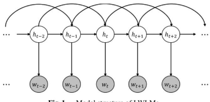
Fig. 1 Model structure of LWLMs.

tent words equals the number of observed words, and multiple LWLMs can share a common latent variable space.

In the generative process of an LWLM, a latent word htis generated on the basis of a transition probability model and its contextlt=ht−n+1,· · ·,ht−1. An observed wordwtis generated on the basis of an emission probability model and a latent wordht. A graphic rendering of LWLM is shown in Fig. 1. The gray circles denote observed words and the white circles denote latent variables. The LWLM produces the generative probability of the observed word sequencew = w1,· · ·, wT. The probability is approximately calculated by the following point estimation:

P(w)

T

t=1

ht∈V

P(wt|ht,Θlw)P(ht|lt,Θlw), (1)

where Θlw indicates a model parameter of the LWLM, andVis the vocabulary. The transition probability model P(ht|lt,Θlw) is expressed as an n-gram model for latent words; it can capture the sentence pattern on the basis of a latent variable sequence. The emission probability model P(wt|ht,Θlw) is expressed as a unigram model for each latent word and can capture the lexical pattern. Usually a hierarchical Pitman-Yor prior is used as the transition probability model, and a Dirichlet prior is used as the emission probability model. More details are provided in previous stud- ies[15]–[18].

2.2 N-gram Mixture Models

N-gram mixture model is constructed by combining sev- eral n-gram LMs trained using diﬀerent sources. A graphic rendering of an n-gram mixture model is shown in Fig. 2;

the model index is represented as zt ∈ {1,· · ·,Z}. Each n-gram LM calculates the generative probability of word wt given context information ut using n −1 words be- hindwt. As shown in Fig. 2, the observed word sequence w=w1,· · ·, wT is generated dependent on model index sequence z = z1,· · ·,zT. The generative probability of the observed word sequencewis defined as:

P(w)=

T

t=1

zt∈{1,···,Z}

P(zt)P(wt|ut,Θ^zng^t ), (2) where P(zt) is the mixture weight for the zt-th n-gram model.

(3)

Fig. 2 Model structure of n-gram mixture models.

In practice, direct implementation of the n-gram mixture model to ASR is not ideal because it does not have a back-oﬀn-gram structure. Actually, the n-gram mixture model can be approximately represented as a single back- oﬀn-gram structure[26].

For domain adaptation of n-gram mixture models, mixture weights are optimized using a validation data set.

The expectation maximization algorithm, which is based on maximum likelihood (ML) criterion, can be used for the optimization[23]. Given a validation data set W = w1,· · ·, w|W|, the optimized mixture weight ˆP(z) is esti- mated in an iterative manner as:

P(z)ˆ = 1

|W|

t=1

P(wt|ut,Θ^zng)P(z)

z∈{1,···,Z}P(wt|ut,Θ^zng)P(z). (3) After iterations, the optimized weight ˆP(z) is used in Eq. (2).

3. Proposed Method

3.1 LWLM Mixture Models

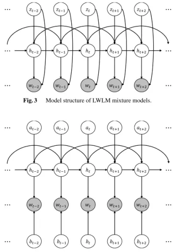
This paper details LWLM mixture models. A graphic rendering of LWLM mixture models is shown in Fig. 3. As shown, LWLM mixture modeling can be considered to be the union of Fig. 1 and Fig. 2. The gray circles denote observed words and the white circles denote latent variables and model indices.

The generative process starts with model index zt ∈ {1,· · ·,Z}, which corresponds to each LWLM index. Then, latent wordht and observed word wt are generated based on the basis of the selected LWLM’s stochastic process. In LWLM mixture models, the generative probability ofwis defined as:

P(w)=

T

t=1

h_t∈V

z_t∈{1,···,Z}

P(wt|ht,Θ^z_lw^t )P(ht|lt,Θ^z_lw^t )P(zt), (4) where Θ^z_lw^t is thezt-th model parameter of the pre-trained LWLM, andP(zt) indicates the mixture weight for thezt-th model. In this equation,P(zt) can be estimated from a validation data set. This equation is based on the characteristics that LWLMs share a common latent variable space.

3.2 LWLM Cross-Mixture Models

This paper also proposes LWLM cross-mixture models. In

Fig. 3 Model structure of LWLM mixture models.

Fig. 4 Model structure of LWLM cross-mixture models.

fact, LWLMs are divided into two components, i.e., a transition probability model and an emission probability model.

Therefore, each component can be independently mixed.

The mixture of transition probability models is performed in the latent variable space, and the mixture of emission probability models is performed in the observed word space. To this end, two model indices are introduced with respect to each component model. A graphic rendering of the LWLM cross-mixture models is shown in Fig. 4.

Its generative process starts when the transition probability model indexat ∈ {1,· · ·,Z}and the emission probability model indexbt ∈ {1,· · ·,Z}are generated independently. Then, latent word ht is generated on the basis of the selected transition probability model and its context lt. Observed wordwt is generated on the basis of the selected emission probability model and latent word ht. In a standard LWLM mixture model,htandwt are generated using the same LWLM, whereas they are generated using diﬀer- ent LWLMs in an LWLM cross-mixture model. In LWLM cross-mixture models, the generative probability ofwis defined as:

P(w)=

T

t=1

h_t∈V

a_t∈{1,···,Z}

b_t∈{1,···,Z}

P(wt|ht,Θ^b_lw^t)P(ht|lt,Θ^a_lw^t)P(at)P(bt), (5)

(4)

using a validation data set.

3.3 Optimization for Domain Adaptation

To optimize mixture weights using a validation data set for domain adaptation, the ML criterion cannot be employed because the latent word sequence is an underspecified variable. If the ML criterion is used, all possible latent word assignments have to be considered since LWLM has a soft clustering structure. It is computationally and analytically intractable to calculate the expectation value. Therefore, this paper employs the Bayesian criterion and a sampling based procedure that is compatible with LWLM training. In the sampling based procedure, model index sequences of the validation data set are estimated for determining the mixture weights.

3.3.1 Optimization of LWLM Mixture Models

In order to optimize the LWLM mixture models, the optimized mixture weight ˆP(z) is estimated using a validation data set W = w1,· · ·, w|W|. In the Bayesian criterion, a model index sequence of the validation data setZ and a latent word sequenceHare estimated using the Gibbs sampling. A conditional probability of possible values for latent wordht∈ Vis given by:

P(ht|W,H−t,Z)∼P(wt|ht,Θ^z_lw^t )

t+n−1

j=t

P(hj|lj,Θ^z_lw^t ), (6) where H₋t represents all latent words except forht. In a similar way, a conditional probability of possible values for model indexzt∈ {1,· · ·,Z}is given by:

P(zt|W,H,Z−t)∼P(wt|ht,Θ_lw^z^t )P(ht|lt,Θ_lw^z^t )P(zt|Z−t), (7) whereZ₋t represents model index sequence except forzt. Gibbs sampling can be used to sample new values for the model index and the latent variable according to these two distributions and place them at positiont.

Once model index sequence is concluded,P(zt|Z) can be calculated as:

P(zt|Z)= c(zt)+β

z∈{1,···,Z}c(z)+βZ, (8)

wherec(zt) denotes the count of model indexztinZ.βis a hyper parameter for Dirichlet distribution.

In a Bayesian criterion, optimized value ˆP(z) is esti- mated by Monte Carlo integration. Multiple model index sequences sampled after the burn-in period are defined as Z¹,· · ·,Z^S. ˆP(z) is estimated as:

ML criterion.

3.3.2 Optimization of LWLM Cross-Mixture Models In LWLM cross-mixture models, optimized mixture weights P(a) and ˆˆ P(b) are simultaneously estimated by defining both model index sequences of a validation data setW. Gibbs sampling can also be used to assign latent word sequenceH, transition probability model index sequenceA, and emission probability model index sequenceBto the validation data setW. The conditional probability of possible values for latent wordht∈ Vis given by:

P(ht|W,H₋t,A,B)∼P(wt|ht,Θ^b_lw^t)

t+n−1

j=t

P(hj|lj,Θ^a_lw^t).

(10) In a similar way, the conditional probabilities of possible values for model indicesat ∈ {1,· · ·,Z}andbt∈ {1,· · ·,Z}

are given by:

Once both assignments are defined, each probability can be calculated.

P(at|A)= c(at)+β

a∈{1,···,Z}c(a)+βZ, (13) P(bt|B)= c(bt)+β

b∈{1,···,Z}c(b)+βZ, (14)

wherec(at) denotes the count of model indexatinA, and c(bt) denotes the count of model indexbtinB,βis a hyper parameter for Dirichlet distribution.

In a Bayesian criterion, optimized values ˆP(a) and ˆP(b) are also estimated by Monte Carlo integration. Multiple model index sequences sampled after the burn-in period are defined asA¹,· · ·,A^S andB¹,· · ·,B^S. ˆP(a) and ˆP(b) are estimated as:

P(a)ˆ = 1 S

S

s=1

P(a|A^s), (15)

P(b)ˆ = 1 S

S

s=1

P(b|B^s). (16)

3.4 Implementation for ASR

In order to implement the LWLM mixture model and the

(5)

Algorithm 1 Random sampling based on LWLM mixture model.

Input:Model parametersΘ¹_lw,· · ·,Θ^M_lw, number of sampled wordsT Output: Sampled wordsw

1: l1=<s>

2: fort=1 toTdo 3: zt∼P(zt) 4: ht∼P(ht|lt,Θ^z_lw^t) 5: w^t∼P(w^t|ht,Θ^zlw^t) 6: end for

7: return w=w1,· · ·, wT

LWLM cross-mixture model to ASR, a special technique is needed as well as a standard LWLM. Therefore, this paper introduces an n-gram approximation technique for both the LWLM mixture model and the LWLM cross-mixture model.

The n-gram approximation is a method that approximates target LM as a simple back-oﬀ n-gram structure, and of- fers one-pass ASR decoding. The n-gram approximation of LWLM mixture model has the following properties:

wlwm ∼ P(w|Θlwm), (17)

wlwmng ∼ P(w|Θlwmng), (18)

wlwm wlwmng, (19)

where wlwm is an observed word sequence generated from the LWLM mixture model, andwlwmngis an observed word sequence generated from the approximated model with back-oﬀn-gram structure.

In a similar way, the n-gram approximation of LWLM cross-mixture model has the following properties:

wlwcm ∼ P(w|Θlwcm), (20)

wlwcmng ∼ P(w|Θlwcmng), (21)

wlwcm wlwcmng, (22)

wherewlwcmis an observed word sequence generated from the LWLM cross-mixture model, andwlwcmngis an observed word sequence generated from approximated model with back-oﬀn-gram structure.

The random sampling of LWLM mixture model is based on Algorithm 1. In addition, the random sampling of LWLM cross-mixture model is based on Algorithm 2. In line 1,l1is initialized as a sentence head symbol<s>. With Titerations,Tlatent words, andT observed words are generated. TheT observed words are used only for back-oﬀ n-gram model estimation.

4. Experiment 1

4.1 Setups

In the first experiment, a target domain data set and an out- of-domain data set were prepared for constructing an LM. In the experiment, the Corpus of Spontaneous Japanese (CSJ) was divided into academic lectures and extemporaneous lectures[27]. Target domain was set to the academic lectures;

Algorithm 2 Random sampling based on LWLM cross- mixture model.

Input: Model parametersΘ¹_lw,· · ·,Θ_lw^M, number of sampled wordsT Output: Sampled wordsw

1: l1=<s>

2: fort=1 toTdo 3: at∼P(at) 4: bt∼P(bt) 5: ht∼P(ht|lt,Θ^alw^t) 6: wt∼P(wt|ht,Θ^b_lw^t) 7: end for

8: returnw=w1,· · ·, wT

Table 1 Experimental data set in Experiment 1.

Domain # of words

Train A Academic lecture 3,468,133 Train B Extemporaneous lecture 3,847,816

Valid Academic lecture 28,046

Test A Academic lecture 27,907 Test B Extemporaneous lecture 18,251

a validation data set (Valid) was prepared for the target domain. Training data sets (Train A and B) and test data sets (Test A and B) were prepared for both domains. Vocabulary size for Train A was 40,725 and that for Train B was 64,543.

Details of the experimental data set are shown in Table 1.

For ASR evaluation, an acoustic model on the basis of hidden Markov models with deep neural networks (DNN- HMM) was prepared[28]. The DNN-HMM had eight hidden layers with 2048 nodes and was trained using the CSJ.

The speech recognition decoder was VoiceRex, a WFST- based decoder[29],[30]. JTAG was used as the morpheme analyzer to split sentences into words[31].

In the evaluation, we aimed to compare following two settings. One setting was that single training data set is only available. Another setting was that multiple training data sets are available. For the former setting, the following base LMs were individually constructed from each training data set.

1. HPY3: Word-based 3-gram hierarchical Pitman-Yor LM (HPYLM) constructed from a training data set[32]. For the training, 200 iterations were used for burn-in, and collected 10 samples. HPY3 constructed from the training data set A is denoted as 1-A, and HPY3 constructed from the training data set B is denoted as 1-B

2. LW3: Word-based 3-gram HPYLM constructed from data generated on the basis of 3-gram LWLM. The generated data size was one billion words which was determined in consideration of previous work[18]. We pruned n-gram entries as to be comparable computation complexity toHPY3 using entropy based pruning[33]. The LWLM was constructed from a training data set. For the training of LWLM, 500 iterations were used for burn-in and collected a sample.LW3con- structed from the training data set A is denoted as 2-A, andLW3constructed from the training data set B is de-

(6)

3-A. HPY3+LW3 65.30 19.27 58.25 21.09 156.45 30.26

1-B. Base model B HPY3 180.02 30.76 127.26 32.24 88.48 24.22

2-B. (Out-of-domain training set) LW3 174.84 30.25 122.44 31.45 90.71 24.30

3-B. HPY3+LW3 161.60 29.20 115.57 30.68 83.20 23.02

4. Adapted model HPYM3 71.68 18.78 64.19 20.34 178.71 26.56

5. ALWM3 72.83 18.56 64.57 20.22 178.48 26.38

6. LWM3 72.72 18.45 64.39 20.10 162.87 25.29

7. HPYM3+ALWM3 67.52 17.88 60.45 19.62 178.53 26.25

8. HPYM3+LWM3 67.38 17.64 60.19 19.36 164.46 25.34

Table 2 Out-of-vocabulary rate [%] in Experiment 1.

OOV rate Vocabulary size Valid Test A Test B

Base model A 40,725 0.89 0.90 3.65

Base model B 64,543 3.59 3.56 1.11

Adapted model 81,856 0.67 0.50 0.94

noted as 2-B.

3. HPY3+LW3: Mixed model which combined HPY3 and LW3with a mixture weight. The mixture weight was set as 0.5 that was an optimal value for the validation set. The mixed model trained from training data set A is denoted as 3-A, and the mixed model trained from training data set B is denoted as 3-B.

Besides, for the latter setting, five adapted LMs which used not only the training data set A but also the training data set B were prepared.

4. HPYM3: HPYLM mixture model consisting of HPYLMs (HPY3) individually constructed from each training data.

5. ALWM3: HPYLM mixture model consisting of n-gram approximated LWLMs (LW3) individually constructed from each training data.

6. LWM3: Word-based 3-gram HPYLM constructed from data generated on the basis of an LWLM mixture model. The LWLM mixture model was constructed from an LWLM trained from the training data set A and an LWLM trained from the training data set B. For the n-gram approximation, one billion words were generated as with LW3. We pruned n-gram entries as to be comparable computation complexity toHPYM3 using entropy based pruning.

7. HPYM3+ALWM3: Mixed model ofHPYM3andALWM3.

8. HPYM3+LWM3: Mixed model ofHPYM3andLWM3.

The vocabulary size for each adapted model was 81,558.

The mixture weights in the adapted models were optimized for the validation data set. For the Monte Carlo integration, S was set to 10. Other hyper parameters were also optimized using the validation data set. Table 2 shows out- of-vocabulary (OOV) rate for both base LMs and adapted LMs.

4.2 Results

Table 3 shows the perplexity (PPL) and word error rate (WER) results for each condition. The diﬀerence of PPL in base models and in adapted models cannot be compared since each vocabulary size diﬀers.

Lines 1-A to 3-A show the results which only used the training data set A, and lines 1-B to 3-B show the results which only used the training data set B. LW3provides results comparable toHPY3 in a same domain, and performs robustly in out-of-domain. The WER diﬀerence between LW3andHPY3in test set B was statistically significant (p<

0.05). The highest performance was obtained byHPY3+LW3.

The WER diﬀerences betweenHPY3andHPY3+LW3in each test set were statistically significant (p < 0.05). It can be considered that the performance was improved becauseLW3 andHPY3had diﬀerent attributes, which observed words are generated depending on latent words inLW3while they are generated depending on last observed words inHPY3.

Next, Lines 4-8 show the results of adapted LMs which used both the training data set A and the training data set B.

The results show performance improvements were obtained by using the out-of-domain training data compared with only using the target domain training data. About the target domain,ALW3MandLWM3provided comparable performance toHPYM3. In addition, both of LWLM-based adapted models acquired the improvement by combining mixture of HPYLMs. It is considered to originate in having the char- acter in whichHPYM3diﬀer fromLWM3. The highest performance was obtained byHPYM3+LWM3. In terms of WER, statistically significant performance improvements (p <0.01) were achieved byHPYM3+LWM3compared toHPYM3.

On the other hand, about the out-of-domain, LWM3 achieved higher performance thanHPYM3andALWM3. The WER diﬀerence between ALWM3 and LWM3 in test set B was statistically significant (p < 0.01). This result shows that mixture modeling in the latent variable space can perform more flexible adaptation than that in the observed word space. Actually, in mixture modeling on a latent variable space, the mixture weight for base model B is comparatively high compared with that in an observed word space. The mixture weight for base model B inALWM3was 0.09 while

(7)

that inLWM3was 0.13. In terms of WER, statistically significant performance improvements (p < 0.01) were also achieved byHPYM3+LWM3compared toHPYM3. It turned out thatLWM3can achieve improvement for both the target domain and the out-of-domain compared withHPYM3.

5. Experiment 2

5.1 Setups

In the second experiment, two types of partially matched training data sets were prepared for constructing an LM. The target domain was set to academic lecture speech; its style is spontaneous speech and the topic is related to acoustics.

A validation data set (Valid) and a test data set (Test) for the target domain were prepared from CSJ[27]. Each data set had about 30K words.

Training data set A (Train A) consisted of transcrip- tions of simulated lecture speeches that are included in CSJ.

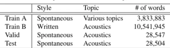
The data size was about 4M words and the style matched that of the target domain but the topic was not related to the target domain. The vocabulary size was 64,761. On the other hand, training data set B (Train B) consisted of Web documents collected using the validation data set based on relevant document retrieval techniques[34]. The data size was about 11M words and the topic was related to the acoustics but the style was written text. The vocabulary size was 64,152. These setups seem to be reasonable for practical spontaneous speech recognition tasks. Details of the experimental data set are summarized in Table 4.

For evaluating ASR performance, a DNN-HMM acoustic model was prepared[28]. The DNN-HMM had 8 hidden layers with 2048 nodes and 3072 outputs.

The speech recognition decoder was a WFST-based decoder[29].

Our experimental settings aimed to compare following two settings. One setting was that single partially matched training data set is only available. Another setting was that multiple training data sets which complement each other are available. For the former setting, four types of base LMs were individually constructed from each training data set.

1. HPY3: Word-based 3-gram HPYLM constructed from a training data set[32]. For the training, 200 iterations were used for burn-in, and collected 10 samples.HPY3 constructed from the training data set A is denoted as 1-A, andHPY3constructed from the training data set B is denoted as 1-B.

2. RNN: Class-based RNNLM with 500 hidden nodes and 500 classes constructed from a training data set[12].

Table 4 Experimental data set in Experiment 2.

Style Topic # of words

Train A Spontaneous Various topics 3,833,883 Train B Written Acoustics 10,541,945

Valid Spontaneous Acoustics 28,547

Test Spontaneous Acoustics 28,504

RNNconstructed from the training data set A is denoted as 2-A, andRNNconstructed from the training data set B is denoted as 2-B.

3. LW3: Word-based 3-gram HPYLM constructed from data generated on the basis of 3-gram LWLM. The generated data size was one billion words which was determined in consideration of our previous work[18].

We pruned n-gram entries as to be comparable computation complexity toHPY3using entropy based pruning[33]. The LWLM was constructed from a training data set. For the training of LWLM, 500 iterations were used for burn-in and collected 10 samples. LW3con- structed from the training data set A is denoted as 3-A, andLW3constructed from the training data set B is denoted as 3-B.

4. HPY3+LW3: Mixed model which combinedHPY3 and LW3with a mixture weight. The mixture weight was set as 0.5 that was an optimal value for the validation set. The mixed model trained from training data set A is denoted as 4-A, and the mixed model trained from training data set B is denoted as 4-B.

Next, for the latter setting, following adapted LMs were constructed using the trained base LMs.

5. HPYM3: HPYLM mixture model constructed from HPY3 trained from the training data set A andHPY3 trained from the training data set B. The mixture weights were optimized using the validation data set.

It was converted into a back-oﬀn-gram structure and implemented in a WFST-based one-pass decoder.

6. RNNM: RNN mixture model constructed from RNN trained from the training data set A and RNNtrained from the training data set B. The mixture weights were optimized using the validation data set.RNNMcannot be converted into WFST format, so single use ofRNNMwas only tested in perplexity evaluation. 1000-best rescor- ing was used whenRNNMwas combined with other LM.

7. LWM3: Word-based 3-gram HPYLM constructed from data generated on the basis of an LWLM mixture model. The LWLM mixture model was constructed from an LWLM trained from the training data set A and an LWLM trained from the training data set B. For the n-gram approximation, one billion words were generated as with LW3. We pruned n-gram entries as to be comparable computation complexity toHPYM3 using entropy based pruning. The mixture weights were optimized using the validation data set.

8. LWCM3: Word-based 3-gram HPYLM constructed from data generated on the basis of an LWLM cross-mixture model. The LWLM cross-mixture model was constructed from an LWLM trained from the training data set A and an LWLM trained from the training data set B. For the n-gram approximation, one billion words were generated as withLW3andLWM3. We pruned n- gram entries as to be comparable computation complexity to HPYM3 using entropy based pruning. The mixture weights were optimized using the validation

(8)

3-A. LW3 239.91 31.09 179.83 35.45

4-A. HPY3+LW3 223.68 29.86 169.93 34.16

1-B. Base model B HPY3 235.91 30.68 273.09 37.33

2-B. (Training set B) RNN 275.23 - 326.31 -

3-B. LW3 207.91 30.05 240.08 36.47

4-B. HPY3+LW3 200.90 28.82 232.93 34.88

5. Adapted model HPYM3 130.30 25.24 119.22 30.33

6. RNNM 126.35 - 118.45 -

7. LWM3 121.60 24.47 113.76 29.84

8. LWCM3 133.85 25.50 123.55 30.48

9. HPYM3+RNNM3 114.15 24.32 106.49 29.40

10. LWM3+LWCM3 116.54 24.06 108.44 29.37

11. HPYM3+LWM3 115.72 24.27 109.26 29.55

12. HPYM3+LWM3+LWCM3 111.90 23.88 105.74 29.20

13. HPYM3+LWM3+LWCM3+RNNM 105.81 23.42 100.82 28.64

Table 5 Out-of-vocabulary rate [%] in Experiment 2.

OOV rate (%) Vocabulary size Valid Test

Base model A 64,761 3.59 3.55

Base model B 64,152 1.77 1.61

Adapted model 100,677 0.83 0.68

data set.

The vocabulary size for each adapted model was 100,677.

Furthermore, combined models of the adapted models were also constructed. For the Monte Carlo integration,S was set to 10. In these settings, other hyper parameters were optimized using the validation data set. Table 5 demonstrates OOV rate for both base LMs and adapted LMs.

5.2 Results

Table 6 shows the PPL and WER results for each condition.

The diﬀerence of PPL in base models and in adapted models cannot be compared since each vocabulary size diﬀers.

Base LMs constructed from training data set A are shown in lines 1-A to 4-A, and those constructed from training data set B are shown in lines 1-B to 4-B. The validation set was linguistically more complicated than the test set so low perplexity could be achieved in the test set. On the other hand, the test set was acoustically more complicated than the validation set, so WERs on the test set were higher than those of the validation set. In addition, training data set B was collected using the validation data set, so perplexity results for the validation set were relatively low compared to the test set. Among the base LMs,LW3provided better results thanRNNandHPY3, and the highest result was achieved byLW3+HPY3for both the base model A and the base model B. These results are in agreement with experiment 1 and previous papers that state that LWLMs oﬀer robust performance in multiple domains[16]–[18]. In both validation set and test set, the WER diﬀerences between LW3+HPY3and HPY3for both training data sets were statistically significant

(p<0.01).

Adapted LMs constructed from the base LMs are shown in lines 5 to 13. They show that each adapted LM was superior to the base LMs in terms of WER, so domain adaptation based on mixture modeling seem to be eﬀective. LWCM3 was relatively weaker than LWM3 although LWM3 did achieve some improvement overHPYM3.

It can be considered that the cross-mixture structure, which makes component parameters partially exchangeable between the base LMs, adversely impacts mixture modeling.

In fact, individual LWLMs were trained by a sampling technique, so latent word space were not universal between LWLMs. It can be expected thatLWCM3is well constructed by increasing number of samples in LWLM training. On the other hand, the highest performance was achieved by LWM3+LWCM3 that combines an LWLM mixture model and an LWLM cross-mixture model although the WER differences between LWM3+LWCM3 toLWM3 were statistically no significant (p > 0.05). This is because an LWLM cross- mixture model has different characteristics than those of a standard LWLM mixture model. Thus, it seems that an LWLM cross-mixture model can mitigate domain mis- matching between the target domain and each training data set. In both validation set and test set, the WER differences betweenLWM3+LWCM3andHPYM3were statistically significant (p <0.05). LWM3+LWCM3demonstrated higher performance than state-of-the-artRNNMin terms of PPL.

In addition, HPYM3+LWM3 outperformed HPYM3 and LWM3. It is considered to originate in having diﬀerent char- acters in which observed words are generated depending on latent words inLWM3while they are generated depending on last observed words inHPYM3. Among WFST-based one- pass decoding results, the highest performance was obtained by HPYM3+LWM3+LWCM3. The WER diﬀerences between HPYM3+LWM3+LWCM3toHPYM3were statistically significant (p < 0.01). In all results, HPYM3+LWM3+LWCM3+RNNMthat fusedHPYM3+LWM3+LWCM3withRNNMin two-pass decoding presented the best performance. In terms of WER, statis-

(9)

tically significant performance improvements (p < 0.05) were achieved byHPYM3+LWM3+LWCM3+RNNMcompared to HPYM3+RNNM in validation set and test set. This indicates thatLWM3+LWCM3could improve the state-of-the-art domain adapted systems that combines n-gram language modeling and RNN language modeling.

6. Conclusions

In this paper, LWLM mixture models and LWLM cross- mixture models were reported to enhance domain adaptation using out-of-domain text resources. Latent variables in LWLMs are represented as specific words that can be selected from the observed word space, so we can realize mixture modeling with consideration of the latent variable space. The LWLM mixture models can perform latent word space mixture that can mitigate a domain mismatch between a target domain and training data sets. Besides, the LWLM cross mixture models that construct a mixture model for each component in LWLMs can utilize partially matched text resources. The proposed models can be optimized using a small amount of target domain data as well as n-gram mixture modeling. Detailed experiments showed that LWLM mixture modeling outperformed n-gram mixture modeling.

In addition, combination of the LWLM cross-mixture model and the LWLM mixture model yielded performance improvements, while using an LWLM cross-mixture model by itself oﬀers little benefit.

References

[1] R. Rosenfeld, “Two decades of statistical language modeling:

Where do we go from here?,” Proceedings of the IEEE, vol.88, pp.1270–1278, 2000.

[2] J.T. Goodman, “A bit of progress in language modeling,” Computer Speech & Language, vol.15, no.4, pp.403–434, 2001.

[3] T. Brants, A.C. Popat, P. Xu, F.J. Och, and J. Dean, “Large language models in machine translation,” Proc. ACL, pp.858–867, 2007.

[4] J.R. Bellegarda, “Statistical language model adaptation: Review and perspectives,” Speech Communication, vol.42, no.1, pp.93–108, 2004.

[5] P. Koehn and J. Schroeder, “Experiments in domain adaptation for statistical machine translation,” Proc. Second Workshop on Statisti- cal Machine Translation, pp.224–227, 2007.

[6] S. Katz, “Estimation of probabilities from sparse data for the language model component of a speech recognizer,” IEEE Transac- tions on Audio, Speech and Language Processing, vol.35, no.3, pp.400–401, 1987.

[7] R.M. Iyer and M. Ostendorf, “Modeling long distance depen- dence in language: topic mixtures versus dynamic cache models,”

IEEE Transactions on Speech and Audio Processing, vol.7, no.1, pp.30–39, 1999.

[8] R. Iyer, M. Ostendorf, and H. Gish, “Using out-of-domain data to improve in-domain language models,” IEEE Signal Process. Lett., vol.4, no.8, pp.221–223, 1997.

[9] G. Foster and R. Kuhn, “Mixture-model adaptation for SMT,” Proc.

Second Workshop on Statistical Machine Translation, pp.128–135, 2007.

[10] B.-J. Hsu, “Generalized linear interpolation of language models,”

Proc. ASRU, pp.136–140, 2007.

[11] X. Liu, M.J.F. Gales, and P.C. Woodland, “Context dependent language model adaptation,” Proc. INTERSPEECH, pp.837–840, 2008.

[12] T. Mikolov, S. Kombrink, L. Burget, J. Cernocky, and S. Khudanpur,

“Extensions of recurrent neural network language model,” Proc.

ICASSP, pp.5528–5531, 2011.

[13] Y. Shi, M. Larson, and C.M. Jonker, “K-component recurrent neural network language models using curriculum learning,” Proc. ASRU, pp.1–6, 2013.

[14] Y. Shi, M. Larson, and C.M. Jonker, “Recurrent neural network language model adaptation with curriculum learning,” Computer Speech & Language, vol.33, no.1, pp.136–154, 2015.

[15] K. Deschacht, J.D. Belder, and M.-F. Moens, “The latent words language model,” Computer Speech & Language, vol.26, no.5, pp.384–409, 2012.

[16] R. Masumura, H. Masataki, T. Oba, O. Yoshioka, and S. Takahashi,

“Use of latent words language models in ASR: a sampling-based implementation,” Proc. ICASSP, pp.8445–8449, 2013.

[17] R. Masumura, T. Oba, H. Masataki, O. Yoshioka, and S. Takahashi,

“Viterbi decoding for latent words language models using Gibbs sampling,” Proc. INTERSPEECH, pp.3429–3433, 2013.

[18] R. Masumura, T. Adami, T. Oba, H. Masataki, S. Sakauchi, and S.

Takahashi, “N-gram approximation of latent words language models for domain robust automatic speech recognition,” IEICE Transac- tion. on Information and Systems, vol.E99-D, no.10, pp.2462–2470, 2016.

[19] S. Goldwater and T. Griﬃths, “A fully Bayesian approach to unsupervised part-of-speech tagging,” Proc. ACL, pp.744–751, 2007.

[20] P. Blunsom and T. Cohn, “A hierarchical Pitman-Yor process HMM for unsupervised part of speech induction,” Proc. ACL, pp.865–874, 1996.

[21] T.R. Niesler and P.C. Woodland, “Combination word-based and cat- egory-based language models,” Proc. ICSLP, vol.1, pp.220–223, 1996.

[22] R.C. Moore and W. Lewis, “Intelligent selection of language model training data,” Proc. ACL, pp.220–224, 2010.

[23] F. Jelinek and R.L. Mercer, “Interpolated estimation of Markov source parameters from sparse data,” pattern Recognition in Prac- tice, pp.381–397, 1980.

[24] G. Casella and E.I. George, “Explaining the Gibbs sampler,” The American Statistician, vol.46, no.3, pp.167–174, 1992.

[25] R. Masumura, T. Asami, T. Oba, H. Masataki, and S. Sakauchi,

“Mixture of latent words language models for domain adaptation,”

Porc. INTERPSEECH, pp.1425–1429, 2014.

[26] A. Stolcke, “SRILM – an extensible language modeling toolkit,” In Proc. ICSLP, vol.2, pp.901–904, 2002.

[27] K. Maekawa, H. Koiso, S. Furui, and H. Isahara, “Spontaneous speech corpus of Japanese,” Proc. LREC, pp.947–952, 2000.

[28] G. Hinton, L. Deng, D. Yu, G.E. Dahl, A. Mohamed, N. Jaitly, A.

Senior, V. Vanhoucke, P. Nguyen, T.N. Sainath, and B. Kingsbury,

“Deep Neural Networks for Acoustic Modeling in Speech Recogni- tion: The Shared Views of Four Research Groups,” Signal Process- ing Magazine, vol.29, no.6, pp.82–97, 2012.

[29] T. Hori, C. Hori, Y. Minami, and A. Nakamura, “Eﬃcient WFST-based one-pass decoding with on-the-fly hypothesis rescor- ing in extremely large vocabulary continuous speech recognition,”

IEEE transactions on Audio, Speech and Language Processing, vol.15, no.4, pp.1352–1365, 2007.

[30] H. Masataki, D. Shibata, Y. Nakazawa, S. Kobashikawa, A. Ogawa, and K. Ohtsuki, “VoiceRex spontaneous speech recognition technology for contact-center conversations,” NTT Technical Review, vol.5, no.1, pp.22–27, 2007.

[31] T. Fuchi and S. Takagi, “Japanese morphological analyzer using word co-occurrence: JTAG,” Proc. COLING/ACL, pp.409–413, 1998.

[32] S. Huang and S. Renals, “Hierarchical Pitman-Yor language models for ASR in meetings,” Proc. ASRU, pp.124–129, 2007.

[33] A. Stolcke, “Entropy-based pruning of backoﬀlanguage models,”

In Proc. DARPA Broadcast News Transcription and Understanding Workshop, pp.270–274, 1998.

(10)

Ryo Masumura received B.E., M.E., and Ph.D. degrees in engineering from Tohoku Uni- versity, Sendai, Japan, in 2009, 2011, 2016, respectively. Since joining Nippon Telegraph and Telephone Corporation (NTT) in 2011, he has been engaged in research on speech recognition, spoken language processing, and natural language processing. He received the Student Award and the Awaya Kiyoshi Science Promo- tion Award from the Acoustic Society of Japan (ASJ) in 2011 and 2013, respectively, the Sendai Section Student Awards The Best Paper Prize from the Institute of Elec- trical and Electronics Engineers (IEEE) in 2011, the Yamashita SIG Re- search Award from the Information Processing Society of Japan (IPSJ) in 2014, the Young Researcher Award from the Association for Natural Lan- guage Processing (NLP) in 2015, and the ISS Young Researcher’s Award in Speech Field from the Institute of Electronic, Information and Communi- cation Engineers (IEICE) in 2015. He is a member of the ASJ, the IPSJ, the NLP, the IEEE, and the International Speech Communication Association (ISCA).

Taichi Asami received B.E. and M.E. degrees in computer science from Tokyo Institute of Technology, Tokyo, Japan, in 2004 and 2006, respectively. Since joining Nippon Telegraph and Telephone Corporation (NTT) in 2006, he has been engaged in research on speech recognition and spoken language processing. He received the Awaya Kiyoshi Science Promotion Award and the Sato Prize Paper Award from the Acoustic Society of Japan (ASJ) in 2012 and 2014, respectively. He is a member of the ASJ, the Institute of Electronics, Information and Communication Engineers (IEICE), Institute of Electrical and Electronics Engineers (IEEE), and the International Speech Communication Association (ISCA).

Takanobu Oba received B.E. and M.E. degrees from Tohoku University, Sendai, Japan, in 2002 and 2004, respectively. In 2004, he joined Nippon Telegraph and Telephone Cor- poration (NTT), where he was engaged in the research and development of spoken language processing technologies including speech recognition at the NTT Communication Science Lab- oratories, Kyoto, Japan. In 2012, he started the research and development of spoken appli- cations at the NTT Media Intelligence Labora- tories, Yokosuka, Japan. Since 2015, he has been engaged in development of spoken dialogue services at the NTT Docomo Corporation, Yokosuka, Japan. He received the Awaya Kiyoshi Science Promotion Award from the Acoustical Society of Japan (ASJ) in 2007. He received Ph. D. (Eng.) degree from Tohoku University in 2011. He is a member of the Institute of Electrical and Electronics Engineers (IEEE), the Institute of Electronics, Information, and Communication Engineers (IEICE) and the ASJ.

tories, where specialized in statistical language modeling for large vocabulary continuous speech recognition. He joined Nippon Telegraph and Telephone Corporation (NTT) in 2004 and has been engaged in the practical use of speech recognition. He received the Maejima Hisoka Award from the Tsushin-bunko Association in 2013, and the 54-th Sato Prize Paper Award from the Acoustic Society of Japan (ASJ) in 2014.

He is a member of the Institute of Electronics, Information and Communi- cation Engineers (IEICE) and the ASJ.

Sumitaka Sakauchi received M.S. degree from Tohoku University in 1995 and Ph.D. degree from Tsukuba University in 2005. Since joining Nippon Telegraph and Telephone Cor- poration (NTT) in 1995, he has been engaged in research on acoustics, speech and signal processing. He is now Senior Manager in the Re- search and Development Planning Department of NTT. He received the Paper Award from the Institute of Electronics, Information and Com- munication Engineers (IEICE) in 2001, and Awaya Kiyoshi Science Promotion Award from the Acoustic Society of Japan (ASJ) in 2003. He is a member of the IEICE and the ASJ.

Akinori Ito received B.E., M.E., and Ph.D.

degrees from Tohoku University, Sendai, Japan.

Since 1992, he has worked with Research Cen- ter for Information Sciences and Education Cen- ter for Information Processing, Tohoku Univer- sity. He was with the Faculty of Engineering, Yamagata University, from 1995 to 2002. From 1998 to 1999, he worked with the College of Engineering, Boston University, MA, USA, as a Visiting Scholar. He is now a Professor of the Graduate School of Engineering, Tohoku Uni- versity. He is engaged in spoken language processing, statistical text processing, and audio signal processing. He is a member of the Acoustic So- ciety of Japan, the Information Processing Society of Japan, and the IEEE.