Dimensions of Synthesized Time Series Data

Dimensions of Synthesized Time Series Data

Soji Ohara

Faculty of Economics, Nara Sangyo University, Ikomagun, Nara-636,Japan

Isao Masaki

Faculty of Letters,

J(

okugakuin University, Shibuya-ku, Tokyo-150, Japan

Wasaburo Unno RIST,l(inki University, Higasi-Osaka, Osaka-577, Japan

(Received Dece1nber 28, 1992)

Abstract

For the construction of standard scales in the determination of fractal dimensions of chaotic systems, we determine empirically dimensions of artificial time series data that are constructed of ftmctions with different periods and some amount of Gaussian noise. Various trajectories of the data in multi-dimensional phase space are investigated in order to study the effect on the determined dimensions of several parameters, i.e. phase-space dimension, time delay, number of data, and inclusion of noise in the da.t.a, etc .. The results of the analysis show among others that the proper position of correlation distance to estimate the fractal dimension is about a half of the amplitude of variation in the data. The fractal dimension D of a chaotic system should better be determined at the position such that the estimated dimension becomes first satulated with increasing the embedding phase-space dimension. At that position, the embedding dimension amounts about 2D

+

1. Noise have considerable effect on the determination of the correlation dimension so that the latter dimension is difficult to predict if noise is mixed more than 0.12 of the rms dispersion of the system variation. Smoothing out of data to minimize the noise effect is neccesary prior to the analysis.

Key Words: Chaos, Fractal dimension, Embedding, Phase space.

1 Introduction

Iu the study of the origin and the st.mcture of observed time variations of chaotic phenomena, the significance of the fractal dimension oecomes more and more recognized. For instance, dimen- sion may well be understood as a state quantity like entropy, if the similarity between the dimen- sion D and the entropy S of the system is de- scribed in the follwing forms (Takens,1981),

D

=

l. ^llll (I" ^lllllll . f(logC¹¹¹(7·)))

m-+oo r--+0 1n - log ^7" (1) and

S =lim( lim

sup(logC~(r)))

⁽²⁾

r--+0 m-+oo 1n - og 1"

where Cm ( 1·) denotes the number of pairs having the distance less than 1· in the embedding space of the dimension m.

In an attempt to describe the degree of disor- der in X-ray observation of Cygnus X-1, Unno et al.( 1990) measured the fractal dimension by use of the Takens delay coordinated vector space in

which scalar time series data are embedded. In so doing, we have used the known chaotic system (Lorenz at tractor with noise) as the reference scale to which observed time variations can be com- pared for estimating the dimension.

This type of analysis could be applied for any chaotic phenomena in which noise is always asso- ciated. But it is not so obvious to know what-

2 Data Functions

Analyses are performed for synthesized time- series data that are described as follows,

+ csin( v'3ti) +Noise. (3) The dimension of the variations given by the above functions is apparently 3, if a,b and c are all nonzero and noise is absent. The dimension is searched using trajectories of time series data that are constructed about 50 discrete data per period 27r.

We have constructed a vector series via

3 Analysis

\Ye have calculated the correlation exponent from the trajectory of the m-dimensional vector,

vm (

^ti), defined in ecp1ation ( 4). The correlation exponent is defined by

D _ dlog Cm(T)

m - _c. Jl _{og T} ' ⁽⁵⁾

where C111 ( T) is the number of pairs of vector poiuts, V¹¹¹(ti) and l!'¹¹¹(tj), of which the mutual distance in m-dimcnsional phase space is less than r. In practice, we estimate the dimensionality, D111 ,

from the gradient of the figure of log Cm ( T2 ) plot- ting against log ^T2.

The value of Dm obtained locally by the nu- merical differentiation is subject to large fluctu- ation. A smoothing procedure by means of the maximum entropy method is applied as follows, the data C,,i(.j = 0, ··, n) is nonnalizcd to be d0 =

ever kiud of effects will be given to the estimated dimension by various chosen parameters such as embedding dimension, time delay, number of data and noise etc.. In the present paper, we intend to put the reference scaling method usen before (Unno et al.1990) on the firm basis, using well- defined time-series data with and without noise.

x(ti

+

(m- 1)r)](i

=

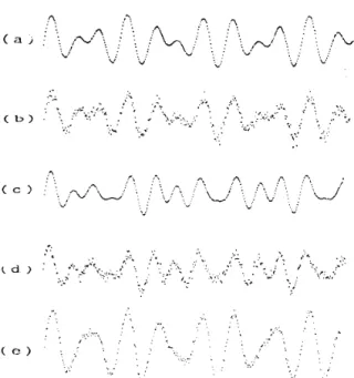
1, 2, 3, · · ·N), (4) where ti = t0 + (i -1), and X(ti) denotes the syn- thesized intensity at time ti, ^T the time delay to construct the vector, m is embedding phase-space dimension, and N the number of data.

In the present study, we analyze the dimen- sion of artificial time-series data synthesized with less than 4 variations. \Ve show in Figure 1 some of the example of the synthesized time-series data (3). Mixed noise is Gaussian noise of given nns dispersion. Each time-series data is constructed of about 50 discrete data per period 27r. Figure 2 shows the delay plots, X(t + r) vs. X(t) for sin

t

+sin

/it

and sin t +sin

/it

+ sin/3t with time delay T to be 5 and 7.

0, d₁·

=

1 by the equation d₁·

=

log c ( _m tnttltmurn Cmi ) and Pi is calculated so that S - Q /). should be maxi- mum (). is a parameter, set to be 1 in the present study), where S

= -

LPj logpj, Q

= "'[;,

dj-

!/

and

fJ = L1=o

Pi.

The procedure is repeated 2 or 3 time 1111-

til small scale flnct nation are eliminated but is stopped before large scale variation is not much altered. In the present study the procedure is re- peated only ouce.

3.1 Embedding dimension

Using the method of Takcns, we calculate the number of pairs Cm(1·) having the distance less than r for several embedding dimensions up to 15.

Figure 3 shows log

C, (

^r2) (continuous line) and Dm for a two dimensional motion, sin t + sin

../2t

.'\ '" ^/'\

( a j

/~,/

\J"""'' . ^/\ ! ^'" v

.. ~

( b )

:·."'

,'\

( c ) : :... .. J'-/"·\..__;/

t d )

( c )

v

\/

·

... ,

\ .. / :.~/ ^....

, ... .,.,_

·~· 't'

~-.;/ ' .

·'

Figure 1: Synthesized time series data.

(a) sin t +sin

/2t

(b) sin t +sin

/2t

+ Noise(0.12) (c) sin t + sin

/2t

^{+ sin}

J3t

(d) sin t +sin V'it +sin

/3t

+ Noise(0.12) (e) 2sin t +sin

/2t

+ Noise(0.08)

... ··

vs. log 1·2 for different embedding dimension, m

\vith keeping time delay r to be 5.

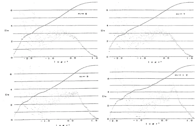
The position of satellite peak of Dm which ap- pears in the Dm(logr²) diagram moves to longer distance region as the embedding dimension m gets to be larger. Similarly, D111(log r²) for sin t + sin V'it + sin y'3t for several embedding dimen- sions are shown in Figure 4. In the region of log 7'2

<

-1.0, D m (log T2

) scatters very widely, while in the region -1.0

<

log ^1·2

<

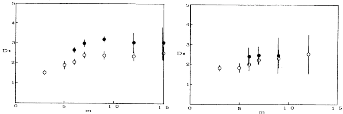
0.0 it is rel- atively stable. In the region longer than 0.0, the rate promptly get to zero because the number of pairs rapidly decreases in this region.

vVe have estimated the dimensionality Dm at two different distance where log ^T2 is -1.0 and 0.0 for several data of Dm calculated under several conditions. Figure 5 shows the dependence of di- mensionality Dm estimated at log r² = 0.0 on 1n

· .. · .

( a )

. .. ·· ...

...

.. :·

:. \f;'.\

:

,.,

.. ,.,.

( b )

Figure 2: Delay plots of synthesized time series data. X(ti) vs. X(ti + r) is plotted for 512 data (a) sin t +sin

/2t (

^r

=

5) and

(b) sin t +sin

/2t

+sin v'3t( r

=

^7).

for 2- D and 3-D variations: sin t + sin V'it and sin t + sin V'it +sin

/3t.

We see that the D₁₁₁(log T2

=

0) value increases with increasing m for small m and becomes first saturated at a bon t m

=

^{2D + 1.} Conversely, for the data of which D is unknown we obtain D

= (

^m -1) /2 from such value of m. On the other hand Figure 6 shows the dependence of Dm esti- mated at log r²

=

-1.0 on m for 2-D and 3-D vari- ations: sin t +sin

J2,t

and sin t +sin

J2,t

+sin

J3t.

The estimated dimension Dm(log ^T2 = -1.0) scat- ters for larger value of m in the former case, and we could not predict correct dimension of variation in the latter case. This result shows that the ap- propriate log 1·2-value should be about log 1·2

=

⁰

for estimating the dimension, D. The appropriate value of r should then be about half of the total amplitude of the given time series data.

m=-"' 5 Do

Do

·,_

o - - - -

- I . 0 0 0

-· 2 0 0 -~---~---~----~

-2 0 - 1 . 0 0.0 1.0

I 0

J o Y. r ,. 1 o p; r ¹

/

/ t t l = Q

2----

0

0 - 2. 0 - 1. 0 ^{0 . 0} I . 0 -- 2 0 - I . 0 0 0 I . 0

1 o K r ¹ 1 0 g ... ¹

Figure 3: log Cm(r²⁾ vs. log r² aud Dm vs. log r² calculated for sin t +sin

/2t

for different embedding dimension in phase space ( m

=

3, 5, 7, 9). Time delay r is kept to be cons taut, 5, and number of data is 512.

Do Do

o---2~.~0---1 .-o----o~.~o---~1 .o

0

Do

---'----2

-~···· ^.. ·.·-~··.~:;:-,

^{... .:__}

_ _

^Do

0 ~-~---1~.~0~---~0~0---~~~-~

1 o g r '

o----,L-L:--= 7

^{n t = 7}

-~---~~---­

/"'

/

----~· -~~---~---­·· .... ,

-~ ... ~.

0 ----::2:-".~o:---=-~ ~. 7o ---o-_'-:o::---~..:1.:--o

1 o P." r '

0

---7'7

^{rn · -1 2}

·---~----

_~/

2~~---~~~~---~----

0~~---~~---~---~

'-2.0 - 1 . 0 o.o I . 0

l o g r '

Figure 4: log Cm ( r2 ) vs. log 1·2 and Dm vs. log r² calculated for sin t + sin

/2t

^{+ sin}

v'3t

for different embedding dimension in phase space (m

=

^6, 7, 9, 12). Time delay r is kept to be constant, 7, and number of data is 512.

s s,---~

4

0

+ ⁺

D•

+ ₉

2

9

9

^¢

0

3

f j

Dm

2 ¢

0 5 1 0

m ^{1 5 0} 5 ^{1 0 1 5}

rrt

Figure 5:

mated

Dependence of dimensionality esti- Figure 6:

mated

Dependence of dimcnsionali ty esti- from Figure 3 and Figure 4 at correlittion distance

log r² = 0.0 i.e. 1· = 1 on the embedding dimen- sion, m. \tVhite circle :sin t +sin .;2t( r = 5 );

black circle :sin t +sin .;2t +sin v'3t( r = i).

3.2 Nutnber of data

\Ve describe next the effects of number of data.

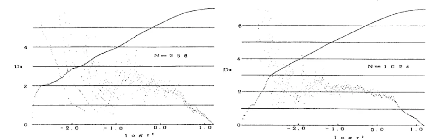
Figure 7 shows Dm (m = 5, r = 5) of sin t+sin .;2t constructed of 256 and 1024 data. The calculated

3.3 Time delay

In Figure 8, we show D₅ for the 2-D variation sin t + sin J2t by changing the time delay ( r =3 and 9). The profiles of Dm of two different condi- tion (m = 5, r = 9) and (1n = 9, r = 5) are quite similar to each other. Generally m and r seem to have similar effect on Dm.

The Dm(log 1·2

) profile shifts to smaller log r²

3.4 Noise

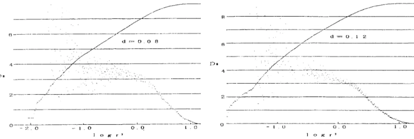
Next, we study the effect of noise on Dm detenni- nations. \tVe shows in Figure 10 several calculated results of Dm for the 2-D variation: sin t +sin .;2t associated with some amount of Gaussian noise . Figure 11 shows Dm(log r²⁾ for the 3-D variation:

sin t +sin

../2t

+sin

/3t.

Dm increases substan- tially in the region of log 7'2

<

0.0.

Since noise shows its dimension to be equal tom, the dimensions depending on smaller ampli- tude variations will be masked by noise. Figure 12

from Figure 3 and Figure 4 at the correlation distance log 7'2 = -1.0 on the embedding dimen- sion, 1n. \Vhi te circle :sin t + sin .;2t ( r = 5);

black circle :sin t +sin .;2t +sin v'Jt( r = 7).

Dm has longer stable log 7'2 span as longer data are employed. We see also that 512 data are nec- essary for the reliability of the present analysis.

So we employ exclusively 512 time-series data (See Figure 3).

as the value of r gets to larger in contrast to the effect of m.

Figure 9 shows the dependence of Dm (log r² = 0.0) on the time delay r for 1n = 5 for the data:

sin

t

^+sin

../2t.

We conclude that the time delay, r, should be taken to be about the same value as the embedding dimension, m for the reliable esti- mation of D.

shows the dependence of Dm(log r² = 0.0) on the amount of mixed Gaussian noise for 2-D and 3-D variations. The dependence of Dm(log 7'2 = -1.0) is shown in Figure 13 for 2-D and 3-D variations.

These results reveal that the influence of noise is negligible if the value of rms dispersion of noise is less than 0.12. But the influence of noise is larger in smaller log r² regions. For instance Dm (log r² = -1.0) can exhibit the the original di- mension D only if the noise is less than 0.04 for sin

t

^+sin

../2t.

We should reduce the noise ampli- tude below some 10

D• D•

;.· ....

0 - - - - _ .,.-2-'--. _o _ _ _ _ -1--'-. -o----=o-.· -=-o---,1~.-:::o•

0---~~----~---~---''_,~~~

''-

2.0 - 1 . 0 0.0 1.0

Figure 7: log Cm ( r²) vs. log r² and Dm vs. log r² ( 1n = 5, r = 5) of sin t + sin

J2t

constructed of 256 and 1024 data.

~

4---~---~-.~~---

. · / T=3

D•

• • 1' . . . .

0 ---_----:2:-' .. ----=oc---:1 o _{0 . 0 1. 0} ) o g r ¹

D•

... ; .:• ''';-:,."

/

2-~/~-.~. --~--~~~~~~~--~~0.-,--- /

,...._

o-~?2--'-.no---~1~.~o~----~o~.~o~---1~.o I o g r 1

Figure 8: logCn(r²) vs. log1·² and Dm vs. logr² (m

=

5) calculated with different r for sint+sin

J2t.

The values of r are 3(1eft) and 9( right) respectively.

5

4

3 ]").

2

+ + +

0 5 1 0 1 5

Time delay

Figure 9: Dependence of dimensionality estimated at log r²

=

0.0 on the time delay for r-;in

t

+sin

J2t.

The embedding dimension is taken to be constant, 5.

Do

Do

---

-~---~---

/ /

~ ---~--~

^•.

-.~-

^{.... -.•.}

--~

^•..•

~

^....

L-~---d-=---o-.-o-2

^{____ __}

/ ^{. .}

r / ...

2

0 2.0 - I . 0 0 0 I . 0

1 o ^K r 1

~----

e----~---~~/~/_/ ________ _

7

^{ct~·o.o s}

4---~--~-r~--- / " /

o.---_ -2-'-. -o ---1--'.'-o---o . o·---~ . -~

1 o g r ¹

7

.v

^d=O.O~

~--

Do

. .·',

/

o---~2~.~0~----~~.~o~----o~.o---~~.~o

1 0 g T t

o--'--~~--

.7 7

d = O . I 2

Do /

.-···'": ....

2 ---~~~---~·~··~·~'~--- .----

0 ---~z~.~o~----~~~.~0---o~.o~---~~.-o~

-

1 o g r'

Figure 10: logC,n(r²) vs. logr² and Dm vs. logr² (m

=

^5,T

=

5) of2-D variation sint+sin.;2t for different mixed Gaussian noise (rms dispersion d

=

0.02, 0.04, 0.08, 0.12).

3.5 Weight of variations

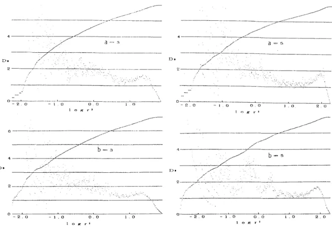
Figure 14 shows D111 for 2-D variation synthe- sized with different weight. The profile of Dm in longer distance area arc greatly influenced by this unevenness of synthesizing. The dependence

4 Discussion

The object of present study is to make clear quantitatively the range of applicability of the method of Takens for determining the fractal di- mension of chaotic time-series phenomena. \Ve have concluded in the first place that the proper correlation distance to determine the fractal di- mension is about half the total amplitude of time- series data. This seems to be due to the fact that the statistics becomes best in the range of log 1·2 ~ 0.0.

For the best determination fractal dimensions

of dimensionality estimated at log r² = 0.0 on the coefficient a and b in a sin t + sin

v'2t

^and

sin t + bsin

V'lt

is shown in Figure 15. These re- sult shows that the dependence of dimensionality on the synthesizing coefficient is negligible if the coefficient is less than 4.

for real chaotic data, therefore, we have to esti- mate it at about half the total amplitude (log r² ~ 0.0) with values of Dm calculated under several embedding dimension, m.

The value of Dm increases with increasing m and then becomes saturated at m. ~ 2D + 1.

Therefore, we can ·conclude that the fractal di- mension D of a chaotic system should better be determined at the position that the estimated di- mension D111(log ^1·2) becomes first saturated with increasing the embedding dimension ,m ,(sec Fig-

---

--z:_~---

. - 7

^{d = 0 0 ~---}

/

n

. /

D11 __________ .£':~~--· - - . - . - · _. ·_· _. -~~:.__--~---

..---

R - - - - -

Do

~//_~ ^{_ _} d_~_-_o_._1_z ^{_ _ _ _ _} ---:/---

/

f l - - - - -

/ /

2 2

o---.1.

- ~~ . 0 ·---~---··'---·_';:o,.._

-· 1. 0 0. () I . 0 0 - I U 0 . 0 I . 0

I o K r ¹

Figure 11: logCm(r²⁾ vs. logr² and Dm vs. logr² (rn = 7,r = 7) of 3-D variation sint + sinv'2t + sin v'3t for different mixed Gaussian noise (rrns dispersion d

=

0.08, 0.12).

r;

'I

:I

• • ^•

u.

,.

¢ ¢ ¢ ¢

0 0 . 0 5

d ^{0. I 0 0. 1 5}

Figure 12: Dependence of dimensionality Dm es- timated at log r²

=

0.0 on the nns dispersion of the mixed Gaussian noise for sin t +sin V2t( m

=

5, r

=

5 )(white circle) and sin t + sin V2t + sin v'3t(m

=

7, r

=

7)(black circle).

[j

4

~

:l

t ^~

Do

~

t

0 . 0 5 0. 1 0

0 0. 1 5

d

Figure 13: Dependence of dimensionality Dm es- timated at log r² = -1.0 on the nus dispersion of the mixed Gaussian noise for sin t +sin v'2t( 1n = 5, r = 5 )(white circle) and sin t + sin v'2t + sin v'3t(m

=

7, r

=

7)(black circle).

-:. ... & - - - -

/_/

/ /

---.-7-----~-

/

Do Do

. /

D•

._,.,.~

2 --~ . . : _ · - - - - , - - - ' ~· ~·. '--;-~-'--- 2 - - _ . , . . _ -

0--.L--_

- 2. 0

6

"

/

2

0 -2. 0

/

' - - - ' - - - " - - - ·

- 1 . 0 o.o 1 n

/

^{b ~ 3}

/ ... ~

; .. , ..

- 1 0 0. 0 I 0

I 0 K r

Do

-·_: ^{',_. '} -~-'

0

- 2 . 0 - I . 0 0 0 I . 0 2 0

2

o--_-27-.o~--~~~.o~-~o~.~o--~~~.o---z~.-o~ \ 1 o P: r ²

Figure 14: log Cm(7·²) vs. log r² and Dm vs. log ^1·2 (m

=

5, ^T

=

5) of a sin t+sin ..f2t and sin t+bsin ..f2t with different value of a and b.

4r---,

4r---~

3 3

Dm

+ ₊

²

^~ + + +

0~----~----L---~----~--~

1 2 3 4

a ^{5 6}

0~----L---~----~----~--~

1 2 3 4

b

^{5 6}

Figure 15: Dependence of dimensionality estimated at log 1·2

=

0.0 on the value of a and b for the time series data a sin

t

+sin

V2t

and sin t + bsin

V2t

(m

=

5, T

=

5).

ure 5). The time interval Tis appropriately taken to be equal to m. Some 512 data points seems to be necessary for reliable determination of D.

The influence of noise is considerably large.

We have estimated the effect of noise so that it

References

is negligible if the dispersion of noise is less than 0.12. These dimensions that are due to smaller amplitude variation are masked by noise. We may reduce the effect of noise by smoothing out the data prior to the analysis ..

(1] Takens,F., 1981, Lecture Notes in Math., 898(Springer-Verlag),366

(2] Unno,W.,Yoneyama,T.,Urata,K.,Masaki,I.,Kondo,!\1. and Inoue,H. 1990,. Astron. Soc. Japan 42, 269-278.