An O(n log 2 n) Algorithm for the Optimal Sink Location Problem in Dynamic Tree Networks
Satoko MAMADA ∗ Takeaki UNO †
Kazuhisa MAKINO ‡ Satoru FUJISHIGE §
Abstract
In this paper, we consider a sink location in a dynamic network which consists of a graph with capacities and transit times on its arcs. Given a dynamic network with initial supplies at vertices, the problem is to find a vertex v as a sink in the network such that we can send all the initial supplies to v as quickly as possible. We present an O(nlog2n) time algorithm for the sink location problem, in a dynamic network of tree structure wherenis the number of vertices in the network. This improves upon the existingO(n2)-time bound. As a corollary, we also show that the quickest transshipment problem can be solved inO(nlog2n)time if a given network is a tree and has a single sink. Our results are based on data structures for representing tables (i.e., sets of intervals with their height), which may be of independent interest.
1. Introduction
We consider dynamic networks that include transit times on arcs. Each arc ahas the transit timeτ(a) specifying the amount of time it takes for flow to travel from the tail to the head ofa. In contrast to the classical static flows, flows in a dynamic network are called dynamic.
In the dynamic setting, the capacity of an arc limits the rate of the flow into the arc at each time instance. Dynamic flow problems were introduced by Ford and Fulkerson [6] in the late 1950s (see e.g. [5]). Since then, dynamic flows have been studied extensively. One of the main reasons is that dynamic flow problems arise in a number of applications such as traffic control, evacuation plans, production systems, communication networks, and financial flows (see the surveys by Aronson [2] and Powell, Jaillet, and Odoni [15]). For example, for building evacuation [7], vertices v ∈ V model workplaces, hallways, stairwells, and so on,
∗Division of Mathematical Science for Social Systems, Graduate School of Engineering Science, Osaka University, Toyonaka, Osaka 560-8531, Japan. E-mail:[email protected]
†Foundations of Informatics Research Division, National Institute of Informatics, Tokyo 101-8430, Japan.
E-mail:[email protected]
‡Division of Mathematical Science for Social Systems, Graduate School of Engineering Science, Osaka University, Toyonaka, Osaka 560-8531, Japan. E-mail:[email protected]
§Research Institute for Mathematical Sciences, Kyoto University, Kyoto 606-8502 Japan. E- mail:[email protected]
and arcsa ∈ Amodel the connection link between the adjacent components of the building.
For an arca= (v, w), the capacityu(a)represents the number of people who can traverse the link corresponding toaper unit time, andτ(a)denotes the time it takes to traverseafromv tow.
This paper addresses the sink location problem in dynamic networks: given a dynamic network with the initial supplies at vertices, find a vertex, called a sink, such that the comple- tion time to send all the initial supplies to the sink is as small as possible. In this setting of building evacuation, for example, the problem models the location problem of an emergency exit together with the evacuation plan for it.
Our problem is a generalization of the following two problems. First, it can be regarded as a dynamic flow version of the 1-center problem [14]. In particular, if the capacities are suf- ficiently large, our problem represents the 1-center location problem. Secondly, our problem is an extension of the location problems based on flow (or connectivity) requirements in static networks, which have received much attention recently [1, 11, 17, 18].
We consider the sink location problem in dynamic tree networks. This is because some production systems and underground passages form almost-tree networks. Moreover, one of the ideal evacuation plans makes everyone to be evacuated fairly and without confusion. For such a purpose, it is natural to assume that the possible evacuation routes form a tree. We finally mention that the multi-sink location problem can be solved by solving the (single- )sink location problem polynomially many times [13]. It is known [12] that the problem can be solved inO(n2)time by using a double-phase algorithm, wheren denotes the number of vertices in the given network. We show that the problem is solvable inO(nlog2n)time.
Our algorithm is based on a simple single-phase procedure, but uses sophisticated data structures for representing tablesg i.e., sets of time intervals[θ1, θ2)with their heightg(θ1) to perform three operations Add-Table (i.e., adding tables), Shift-Table (i.e., shifting a table), and Ceil-Table (i.e., ceiling a table by a prescribed capacity). We generalize interval trees (standard data structures for tables) by attaching additional parameters and show that using the data structures, we can efficiently handle the above-mentioned operations. Especially, we can merge tablesgi inO((idi) log2(idi)) time, where we say that tablesgi are merged if gi’s are added into a single table g after shifting and ceiling tables are performed, and di denotes the number of intervals ingi. This result implies anO(nlog2n)time bound for the location problem. We mention that our data structures may be of independent interest and useful for some other problems which manage tables.
We remark that our location problem for general dynamic networks can be solved in poly- nomial time by solving the quickest transshipment problemntimes. Here the quickest trans- shipment problem is to find a dynamic flow that zeroes all given supplies and demands within the minimum time, and is polynomially solvable by an algorithm of Hoppe and Tardos [9].
However, since their algorithm makes use of submodular function minimization [10, 16] as a subroutine, it requires polynomial time of high degree. As a corollary of our result, this paper shows that the quickest transshipment problem can be solved inO(nlog2n)time if the given network is a tree and has a single sink.
The rest of the paper is organized as follows. The next section provides some preliminaries and fixes notation. Section 3 presents a simple single-phase algorithm for the sink location problem, and Section 4 describes and discusses our data structures. In Section 5, we analyze
the complexity of our single-phase algorithm with our data structures. Finally, we give some conclusions in Section 6.
2. Definitions and Preliminaries
LetT = (V, E) be a tree with a vertex set V and an edge set E. Let N = (T, c, τ, b) be a dynamic flow network with the underlying undirected graph being a treeT, wherec : E → R+is a capacity function representing the least upper bound for the rate of flow through each edge per unit time,τ :E → R+ a transit time function, andb :V → R+ a supply function.
Here,R+denotes the set of all nonnegative reals and we assume the number of vertices inT is at least two.
This paper addresses the problem of finding a sink t ∈ V such that we can send given initial suppliesb(v) (v ∈V \ {t})to sinktas quickly as possible. Suppose that we are given a sink t inT. Then, T is regarded as an in-tree with root t, i.e., each edge ofT is oriented toward the roott. Such an oriented tree with roott is denoted by T(t) = (V, E(t)). Each oriented edge in E(t) is denoted by the ordered pair of its end vertices and is called an arc.
For each edge {u, v} ∈ E, we writec(u, v)and τ(u, v) instead of c({u, v})and τ({u, v}), respectively. For any arce∈E(t) and anyθ∈R+, we denote byfe(θ)the flow rate entering the arce at timeθ which arrives at the head ofeat timeθ+τ(e). We callfe(θ)(e ∈ E(t), θ ∈ R+) a continuous-time dynamic flow inT(v∗)(with a sinkv∗) if it satisfies the following three conditions, whereδ+(v)andδ−(v)denote the set of all arcs leavingv and enteringv, respectively.
(a) (Capacity constraints): For any arce∈E(t) andθ ∈R+,
0≤fe(θ)≤c(e). (2.1)
(b) (Flow conservation): For anyv ∈V \ {v∗}andΘ∈R,
e∈δ+(v)
Θ
0 fe(θ)dθ−
e∈δ−(v)
Θ
τ(e)fe(θ−τ(e))dθ ≤b(v). (2.2) (c) (Demand constraints): There exists a timeΘ∈R+such that
e∈δ−(v∗)
Θ
τ(e)fe(θ−τ(e))dθ−
e∈δ+(v∗)
Θ
0 fe(θ)dθ =
v∈V\{v∗}
b(v). (2.3)
As seen in (b), we allow intermediate storage (or holding inventory) at each vertex. For a continuous-time dynamic flowf, letθf be the minimum time θ satisfying (2.3), which is called thecompletion time forf. We further denote by C(v∗)the minimum θf among all continuous dynamic flows f in T(v∗). We study the problem of computing a sink v∗ ∈ V with the minimumC(v∗). This problem can be regarded as a dynamic version of the 1-center location problem (for a tree) [14]. In particular, ifc(v, w) = +∞(a sufficiently large real) for each edge{v, w} ∈E, our problem represents the 1-center location problem [14].
We remark that dynamic flows can be restricted to those having no intermediate storage without changing optimal sinks of our problem (see discussions in [6, 9, 12], for example).
2.1. An O(n
2) algorithm given in [12]
In this section, we review the outline of anO(n2)algorithm which has been proposed in [12], in order to make our faster algorithm easily understood.
The algorithm consists of two phases, Phases I and II. Phase I arbitrarily chooses a vertex t ∈ V as a candidate sink and compute the completion timeC(t)and a dynamic flowf that completes inC(t). Then Phase II computes an optimal sinkt∗by repeatedly picking up a new candidate sinkˆtthat is adjacent to the current onetand updatingt:= ˆtifC(ˆt)< C(t).
In both phases, we keep two tables, Arriving Table Av and Sending Table Sv for each vertexv ∈V. Arriving TableAv represents the sum of the flow rates arriving at vertexv as a function of timeθ, i.e.,
e∈E(t):e=(u,v)
fe(θ−τ(e)) +ηθ(v), (2.4) wherefe(θ) = 0holds for anye∈E(t) andθ <0, andηθ(v) = b(∆v) if0≤θ < ∆; otherwise 0. Here,∆denotes a sufficiently small positive constant. Intuitively,ηθ(v)denotes the initial supply atv Sending TableSv represents the flow rate leaving vertexv as a function of timeθ, i.e.,
f(v,w)(θ), (2.5)
where(v, w)∈E(t).
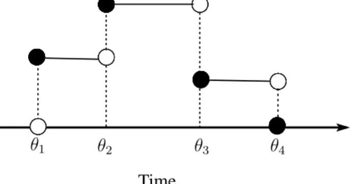
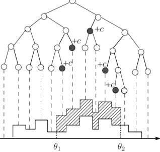
Let us consider a table g : R+ → R+ , which represents the flow rate in time θ ∈ R+. Here, we assume g(θ) = 0 for θ < 0. Since our problem can be solved by sending out as much amount of flow as possible from each vertex to its parent if a candidate sinktis chosen in advance, we only consider the tableg which is representable as
g(θ) =
0 ifθ < θ1
g(θi) ifθi ≤θ < θi+1 fori= 1,· · ·, k−1 0 ifθ ≥θk,
(2.6)
whereθi < θi+1 andg(θi) = g(θi+1)fori = 1, . . . , k. Thus, we represent such tables g by a set of intervals (with their height), i.e.,
((−∞, θ1),0), ([θi, θi+1), g(θi)) (i= 1,2,· · ·, k), (2.7) whereθk+1 = +∞andg(θk) = 0. A timeθis called ajump timeofgiflimx→−0g(θ+x)= limx→+0g(θ+x).
Figure 1 shows such a tableg, where black circles denoteg(θi)’s at jump timeθi’s.
Let us now describe Phases I and II as follows.
Algorithm DOUBLE-PHASE
(Phase I)
Step 0: Choose a vertextarbitrarily. PutT ←T(t).
Step 1: IfT consists oftalone, then go to Step 3. For each leafv ofT, construct Sending Sv from Arriving TableAvby boundingAv byc(v, w), wherewis a parent ofv inT.
θ1 θ2 θ3 θ4
Time
Figure 1: An example of a table that can be decomposed into intervals.
Step 2: For each internal nodewwhose children are all leaves, construct Arriving TableAw from Sending TablesSv of its childrenv by shiftingAv right byτ(v, w)and adding all such shifted tables and the initial supplyηθ(w).
Remove all the leavesv(=t)fromT and denote the resultant tree byT again.
Go to Step 1.
Step 3: Compute the completion timeC(t)fromAt. (Phase II)
Step 0: Find a childv of roott that sends the last flow tot(i.e., the flow that arrives at time C(t)). Putˆt ←v and considerˆtas a new sink. Ifv is not unique, thent∗ =tand halt.
Step 1: Compute the completion timeC(ˆt)and the corresponding tables as follows.
(1-1) Compute new Arriving Table A˜tby subtracting fromAtthe table obtained from Sˆtby shifting it right byτ(ˆt, t).
(1-2) Compute from new A˜t Sending Table St to go through (t,ˆt) (as in Step 1 of Phase I).
(1-3) Compute new Arriving TableA˜ˆtby addingAˆtand the table constructed fromSt
by shifting it right byτ(t,ˆt). Compute the completion timeC(ˆt).
Step 2:
(2-1) IfC(t)< C(ˆt), then returnt∗ =tand halt.
(2-2) IfC(t)≥C(ˆt)and the last flow reaches sinkˆtfromt, then returnt∗ = ˆtand halt.
(2-3) Otherwise, putt ←ˆtand go to Step 0. 2
Note that tables Av and Sv can be constructed by adding, shifting, and/or bounding the other tables. Now, we more formally describe how to compute them.
In Step 1 of Phase I, Arriving TableAv for a leafv of the originalT(t)is given as
((−∞,0),0), ([0,∆), b(v)/∆), ([∆,+∞),0), (2.8) and Sending Table Sv for a leaf v of T can be constructed from Av as follows. Let Av be represented as
((−∞, θ1),0), ([θi, θi+1), hi) (i= 1,2,· · ·, k), whereθk+1 = +∞andhk= 0, and letRi = (hi−c(v, p(v)))(θi+1−θi).
Step 1: Output((−∞, θ1),0)andi:= 1
Step 2: If Ri < 0, then output ([θi, θi+1), hi), and i := i + 1. Otherwise, let α be the index such thatj=iR ≥ 0for any j ≤ α−1and α=iR < 0 and letβ = θα +
α−1
=i R/(c(v, p(v))− hα). Then output ([θi, β), c(v, p(v))) and([β, θα+1), hα), and i:=α+ 1.
Step 3: Ifi=k+ 1, then halt. Otherwise, go to Step 2.
Step 2 of Phase I computes Arriving TableAwfromSv for childrenv’s ofwand the initial supply ofwas follows.
For a childv ofw, letSvbe represented as
((−∞, θ1v),0), ([θiv, θi+1v ), hvi) (i= 1,2,· · ·, kv),
whereθkvv+1 = +∞andhvkv = 0, and let the initial supply ofwbe represented as in (2.8):
((−∞,0),0), ([0, b(w)/∆),∆), ([b(w)/∆,+∞),0).
From these tables, we first sort all the elements in
v:a child ofw
{θvi +τ(v, w) | i = 1,· · ·, kv + 1} ∪ {0, b(w)/∆,+∞}asθ1 < θ2 <· · ·< θk+1(= +∞), and then output((−∞, θ1),0)and
[θi, θi+1),
v:a child ofw
hv(θi−τ(v, w)) + hw(θi) (i= 1,2,· · ·, k),
wherehv(θ)andhw(θ)denote the height of the tableSv and the initial supply ofwat timeθ, respectively.
By using similar methods, Phase II computes the tables.
It was shown in [12] that Algorithm DOUBLE-PHASEcorrectly computes an optimal sink and it requiresO(n2)time. The latter follows from the fact that each tableg can be computed in time linear in the total number of intervals in the tables from whichg is constructed and the number of intervals in each table is linear inn.1 Namely, we have the following theorem.
Theorem 2.1 ([12]): Algorithm DOUBLE-PHASE solves the sink location problem inO(n2)
time. 2
3. A Single-Phase Algorithm
Algorithm DOUBLE-PHASE consists of two phases. This section presents a simple O(n2) algorithm with a single phase. Because of the simplicity, it gives us a good basis for develop- ing a faster algorithm. In fact, we can construct anO(n)˜ algorithm based on this framework, which is given in the next section.
Intuitively, our single-phase algorithm first constructs Sending Table Sv for each leaf v to send b(v) to its adjacent vertex. Then the algorithm removes a leaf v∗ fromT such that the completion time ofSv is the smallest, sinceT has an optimal sink other thanv∗. If some vertex v becomes a leaf of the resulting tree T, then the algorithm computes Sending Table Sv to send all the supplies that have already arrived at v to an adjacent vertex p(v) of the resulting tree T, by using Sending Tables for the verticesw(= p(v))that are adjacent to v in the original tree. The algorithm repeatedly applies this procedure toT untilT becomes a single vertext, and outputs such a vertextas an optimal sink.
1It was shown in [12] that the number of intervals is at most3nfor discrete-time dynamic flows.
Algorithm SINGLE-PHASE
Input: A tree networkN = (T = (V, E), c, τ, b).
Output: An optimal sinktthat has the minimum completion timeC(t)among all vertices of T.
Step 0: Let W := V, and let L be the set of all leaves of T. For each v ∈ L, construct Arriving TableAv.
Step 1: For eachv ∈L, construct fromAv Sending TableSv to go through(v, p(v)), where p(v)is an only vertex adjacent tov inT. Compute the time Time(v, p(v))at which the flow based onSv is completely sent top(v).
Step 2: Compute a vertexv∗ ∈ L minimizing Time(v, p(v)), i.e., Time (v∗, p(v∗))= minv∈L
Time (v, p(v)). LetW :=W \ {v∗}andL:=L\ {v∗}.
If there exists a leafvofT[W]such thatv is not contained inL, then:
(1) LetL:=L∪ {v}.
(2) Construct Arriving TableAv from the initial supplyηθ(v)and Sending TableSv
for the vertices v that are adjacent to v in T and have already been removed fromW.
(3) Compute from Av Sending Table Sv to go through (v, p(v)) where p(v) is a vertex adjacent tovinT[W], and compute Time(v, p(v)).
Step 3: If|W|= 1, then outputt ∈W as an optimal sink. Otherwise, return to Step 2. 2 Here T[W] denotes a subtree of T induced by a vertex set W, and tables Av and Sv are constructed as in Algorithm DOUBLE-PHASE.
Note that at most one leafv ofT[W]is not contained inLin the if-statement of Step 2, andL is always the set of all leaves ofT[W]before executing Step 2 in each iteration. By removing edge (v, w) from T, T is partitioned into two disjoint trees. We denote the one includingv byT(v,w) and by T(+v,w) the trees obtained by addingT(v,w) to edge (v, w). Then we can see that Time(v, p(v))in Step 1 or 2 represents the completion time for−→
T(+v,p(v))(p(v)).
Lemma 3.1: Algorithm SINGLE-PHASEoutputs an optimal sinkt.
Proof. We assume that a vertexu(= t) is an optimal sink. Here, letwbe a vertex adjacent to t on the path fromu to t. We denote byk1, k2 andk3 the completion time for −→
T(t,w)(t),
−→T(+t,w)(w) and−→
T(+w,t)(t), respectively. Then we havek2 = Time(t, w)and k3 = Time(w, t) (see Figure 2).
It follows from the definitions that
k1 ≤k2, C(t) = max{k1, k3}, C(u)≥k2. (3.1) Note thatk3 was chosen ask3 =Time(w, t) = minv∈LTime(v, t)in Step 2 of the algorithm.
This impliesk3 ≤k2, which together with (3.1) impliesC(t)≤C(u). Hencetis also optimal
sinceuis optimal. 2
Similarly as Algorithm DOUBLE-PHASE, it is not difficult to see that Algorithm SINGLE- PHASE requiresO(n2)time if we construct Arriving and Sending Tables explicitly. In Sec- tion 4, we present a method to represent these tables implicitly, and develop anO(nlog2n) time algorithm for our location problem.
t w u T(t,w)
T(+t,w)
T(+w,t)
Figure 2: T(t,w),T(+t,w), andT(+w,t).
4. Implicit Representation for Arriving and Sending Tables
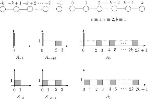
Algorithm DOUBLE-PHASE and SINGLE-PHASE requireΘ(n2)time if explicit representa- tions are used for tables. For example, Figure 3 shows such a network N = (T = (V, E), c, τ, b),
−k −k+ 1−k+ 2 · · · −2 −1 0 1 2 k−2 k−1 k
c≡1, τ ≡2, b≡1
· · ·
0 A−k
0
A−k+1
2 3 0
A0
2 3 4 5 2k 2k+ 1
· · ·
· · ·
0 S−k
1
1 1
1
0 S−k+1
1 1
2 3 0
S0
2 3 4 5 2k 2k+ 1
· · ·
· · · 1
1
Figure 3: A dynamic network that achievesΘ(n2)time bound for our location problem.
whereV ={−k,−k+1,· · ·, k},E ={(i, i+1)|i=−k,· · ·, k−1},c(e) = 1andτ(e) = 2 for alle∈E, andb(v) = 1for allv ∈V. It follows from the symmetry ofT that0is a unique optimal sink. Both Arriving TableAj and Sending TableSj constructed by SINGLE-PHASE
algorithm have2(k− |j|) + 3intervals. Thus the total size of the tables is 2× k
j=−k
2(k− |j|) + 3= 4k2+ 12k+ 6 =n2+ 4n+ 1.
This shows that Algorithm SINGLE-PHASErequiresΘ(n2)time if explicit representations are used for the tables. Similarly, Algorithm DOUBLE-PHASErequiresΘ(n2)time in such a case.
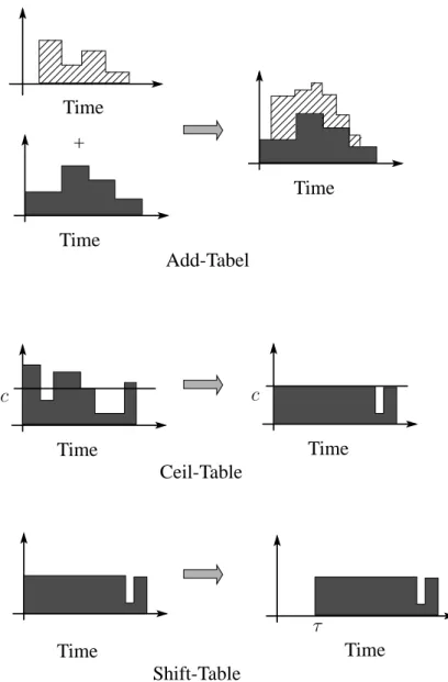
Therefore, we need sophisticated data structures which can be used to represent Arriv- ing/Sending Tables implicitly. We adopt interval trees for them, which are standard data structures for a set of intervals. Note that SINGLE-PHASE only applies to tables Av and/or Sv the following three basic operations (see Figure 4) : Add-Table (i.e., adding tables), Shift- Table (i.e., shifting a table), and Ceil-Table (i.e., ceiling a table by a prescribed capacity). It is known that interval trees can efficiently handle operations Add-Table and Shift-Table (see Section 4.1). However, standard interval trees cannot efficiently handle operation Ceil-Table.
This paper develops new interval trees which efficiently handle all the three operations.
Time Time
Time +
Add-Tabel
Time c
Time c
Ceil-Table
Time Time
τ
Shift-Table
Figure 4: 3 basic operations
4.1. Data Structures for Implicit Representation
This section explains our data structure for representing tables which is obtained from interval tree by attaching several parameters to handle the three operations efficiently. Letg be a table represented as
Ii = ([θi, θi+1), g(θi)) (i= 0,1,· · ·, k), (4.1) whereθ0 = −∞, θk+1 = +∞, andg(θ0) = g(θk) = 0,2and letBTg denote a binary tree for g. We denote the root byrBT and the height ofBT by height(BT). The binary treeBTg has an additional parametertbase to represent how muchg is shifted right. Thistbase is used for operation Shift-Table by updatingtbasetotbase+µ, whereµdenotes the time to shift the table right. Moreover, each nodexinBTg has five nonnegative parameters base(x), ceil(x),he(x), tr(x), andtl(x)withtl(x)≤tr(x), and each leaf hase(x)in addition, where these parameters will be explained later. A leaf xis called active iftl(x) < tr(x)and dummy otherwise. The time intervals of a tableg correspond to the active leaves ofBTg bijectively. We denote by
#(BT)the number of active leaves ofBT.
Initially (i.e., immediately after constructingBTg by operation MAKETREEgiven below), BTg contains no dummy leaf and hence there exists a one-to-one correspondence between the time intervals ofg and leaves ofBTg. Moreover, for each leafxcorresponding toIi in (4.1), we havetl(x) = θi, tr(x) = θi+1,base(x) =g(θi)andceil(x) = +∞, and for each internal nodex,tl(x)=miny∈Leaf(x)tl(y),tr(x)=maxy∈Leaf(x)tr(y),base(x) = 0andceil(x) = +∞. Here, Leaf(x) denotes the set of all leaves which are descendants ofx. Namely, tl(x) and tr(x), respectively, represent the start and the end points of the interval corresponding tox, andbase(x)andceil(x), respectively, represent the flow rate and the upper bound for the flow rate in the time interval corresponding tox.
Operation MAKETREE(g: table) Step 1: Lettbase := 0.
Step 2: Construct a binary balanced treeBTgwhose leavesxi correspond to the time interval Ii ofg in such a way that the leftmost leaf corresponds to the first intervalI0, the next one corresponds to the second intervalI1, and so on.
Step 3: For each leafxi corresponding to intervalIi = [θi, θi+1),base(x) := g(θi), tl(x) :=
θi andtr(x) :=θi+1.
Step 4: For each internal nodex,base(x) := 0, andtl(x) := miny∈Leaf(x) tl(y)andtr(x) :=
maxy∈Leaf(x) tr(y).
Step 5: For each nodex,ceil(x) := +∞.
Step 6: For each leafx, sete(x), and for each nodex, sethe(x), where e(x)andhe(x)shall
be explained later. 2
We can easily compute a tablegfromBTg constructed by MAKETREE. It should also be noted that a binary treeBTg is not unique, i.e., distinct trees may represent the same tableg.
As mentioned in this section, Shift-Table can easily be handled by updatingtbase. We now consider Add-Table, i.e., constructing a table g by adding two tables g1 and g2, where we
2For simplicity, we write the first intervalI0as([−∞, θ1),0)instead of((−∞, θ1),0).
regard an addition ofktables ask−1successive additions of two tables. Let us assume that
#(BTg1)≥#(BTg2), that is,g1has at least as many intervals asg2. Our algorithm constructs BTgby adding all intervals (corresponding to active leaves) ofBTg2 one by one toBTg1. Each addition of an interval([θ1, θ2), c)toBTg1, denoted by ADD(BT1;θ1, θ2, c), can be performed as follows.
We first modifyBTg1 to BTg1 that has (active) leavesx and y such that tl(x) = θ1 and tr(y) = θ2 if there exist no such leaves, as shown in Figure 5. Then we add an interval ([θ1, θ2), c)to the resultingBTg1. One of the simplest way is to addcto all leaves of BTg1 such that the corresponding intervals are included in[θ1, θ2). However, this takesO(n)time, sinceBTg1 may haveO(n)such intervals. We therefore addconly to their representatives.
θ1 θ2
BTg1 BTg1
θ1 θ2
Figure 5: Modification ofBTg1.
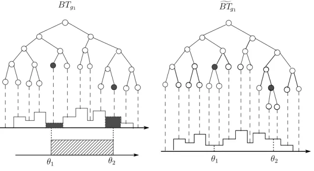
Note that the time interval [θ1, θ2) can be represented by the union of disjoint maximal intervals in BTg1, i.e., the set of incomparable nodes in BTg1, denoted by rep(θ1, θ2) (see Figure 6). We thus updatebase ofBTg1 as follows
base(x) :=base(x) +c for allx∈rep(θ1, θ2). (4.2) We remark that this is a standard technique for interval tree. By successively applying this procedure to new interval tree BTg1 and each of the remaining intervals in BTg2, we can constructBTgwithg =g1+g2.
For an interval treeBTand an active leafxofBT, lety1(=x), y2,· · ·, ys(=rBT)denote the path fromxto the rootrBT. The procedure given above shows that the height of an active leafxrepresenting the flow rate of the corresponding interval can be represented as
h(x) =s
i=1
base(yi). (4.3)
Operation ADD(BTg1;θ1, θ2, c)can be handled inO(height(BTg1)) time, since|rep(θ1, θ2)| ≤ 2height (BTg1). This means thatBTgcan be constructed fromBTg1 andBTg2 inO (#(BTg2)
θ1 θ2 +c +c
+c +c
+c
Figure 6: Black nodes representrep(θ1, θ2).
logn)time by taking balancing of the tree after each addition.Moreover, operations Add-Table in Algorithm SINGLE-PHASE can be performed inO(nlog2n)time in total, since we always add a smaller table to a larger one (see Section 4.3 for the details). Thus Add-Table can be performed efficiently.
However, operations Ceil-Table in Algorithm SINGLE-PHASErequireΘ(n2)time in total, since the algorithm containsΘ(n)Ceil-Table, each of which requiresΘ(n)time, even if we use interval trees as data structures for tables (see Figure 4 for example). Therefore, when we boundBT by a constantc, we omit modifying tl,tr, and base, and keepcasceil(rBT) = c.
Clearly, this causes difficulties to overcome as follows.
First,h(x)in (4.3) does not represent the actual height any longer. Roughly speaking, the actual height iscifc ≤ h(x), andh(x), otherwise. We callh(x)the tentative height of xin BT, and denote byˆh(x)the actual height ofx. Ifcis small, some adjacent intervals can have the same height. In this case, there exists no one-to-one correspondence between active leaves and intervals, and hence we have to merge these intervals into a single one. We will explain how to handle this later.
Let us consider a scenario that an interval([θ1, θ2), c)is added toBT after bounding it by c. Letxbe an active leaf such that (i) the corresponding interval is contained in[θ1, θ2)and (ii) the actual height isc, immediately after boundingBT byc. Then we note that the actual height ofxisc+c after the scenario, which is different from bothh(x)andc. To deal with such scenarios, we updateceil to compute the actual height ˆh(x)efficiently (See more details in the subsequent sections). The actual heightˆh(x)can be computed as
ˆh(x) =h(x)− max
y∈path(x,rBT){0,
z∈path(x,y)
base(z)−ceil(y)}, (4.4)
where path(x, y) denotes the path from x to y. Intuitively, for a node yk in BT, ceil(yk) represents the upper bound of the height of active leavesx ∈ Leaf(yk)within the subtree of BT whose root is yk. Thus ki=1base(yi)−ceil(yk) has to be subtracted from the height h(x)if ki=1base(yi)−ceil(yk) > 0, and the actual heighth(x)ˆ is obtained by subtracting
their maximum. Note thatˆh(x) = h(x)holds for all active leavesxof a tree constructed by MAKETREE.
We next note that there exists no one-to-one correspondence between active leaves inBT and time intervals of the table thatBT represents, if we just set ceil(rBT) = c. See Figure 4, for example. In this case, the table is updated too drastically to efficiently handle the operations afterwards. Thus by modifyingBT (as shown in the subsequent subsections), we always keep the one-to-one correspondence, i.e., the property that any two consecutive active leavesxandx satisfy
ˆh(x)= ˆh(x). (4.5)
We finally note that, for an active leaf x, tl(x) and tr(x) do not represent the start and the end points of the corresponding interval. Let x be an active leaf in BT that does not correspond to the first interval or the last interval. For such anx, letx−andx+denote active leaves inBT which are left-hand and right-hand neighbors ofx, respectively, i.e.,
tr(x−) =tl(x), tl(x+) =tr(x). (4.6) Then the start and the end points of the corresponding interval can be obtained by
ˆtr(x) = tbase+tr(x) + (tr(x)−tl(x))× h(x)−ˆh(x)
ˆh(x)−ˆh(x+) (4.7)
ˆtl(x) = ˆtr(x−). (4.8)
Hereˆtr(x)andˆtl(x)are well-defined from (4.5). For active leavesxandycorresponding to the first interval and the last interval, we haveˆtl(x) =−∞,ˆtr(x) =tl(x+),ˆtl(y) = ˆtr(y)and ˆtr(y) = +∞.
It follows from (4.4), (4.7), and (4.8) that ˆh(x), ˆtr(x), and ˆtl(x) can be computed from base, ceil, tr(x), and tl(x)inO(height(BT))time. In order to check (4.5) efficiently, each active leafxhas
e(x) =
max{0, h(x)−h(x+)} ×tr(x+)−tr(x)
tr(x+)−tl(x) ifx+ exists,
+∞ otherwise
(4.9)
and each nodexhas
he(x) = max
y∈LeafA(x){
z∈path(x,y)
base(z)−e(y)}, (4.10) where LeafA(x) denotes the set of active leaves that are descendants of x, and path(x, y) denotes the set of nodes on the path fromxtoy. As can be seen from Figure 7, we have the following lemma.
Lemma 4.1: Let BT be a binary tree in whichˆh(x) = ˆh(x+)holds for every active leaf x.
After boundingBT by a constantc,
(i) ˆh(x)= ˆh(x+)holds for an active leafxif and only ifxsatisfiesh(x)−e(x)< c, (ii) all active leavesxinBT satisfyh(x)ˆ = ˆh(x+)if and only ifhe(rBT)< c.
Moreover, we can compute an active leafxwithh(x) = ˆˆ h(x+)inO(height(BT))time by scanninghe(x)from the rootrBT. Note thathe(x)can be obtained by the following bottom-up computation.
he(x) =
base(x)−e(x) ifxis a leaf
max{he(x1), he(x2)}+base(x) otherwise, (4.11) wherex1andx2 denote the children ofx. This means that preparing and updatinghe’s can be handled efficiently.
tl(x)
e(x)
tr(x) x x+
tl(x) tr(x) x x+
tˆr(x) h(x)
ˆh(x)
Figure 7: e(x)andt(x).ˆ
In summary, we always keep the following conditions for binary trees BTg to represent tablesg. Note thatBT satisfies the conditions.
(C0) For any nodex,BT maintainstl(x), tr(x), ceil(x), base(x), andhe(x). For any leafx, BT maintainse(x)in addition.
(C1) Any nodexsatisfiestl(x)≤tr(x). Any internal nodexsatisfiestl(x) = miny∈Leaf(x)tl(y), andtr(x) = maxy∈Leaf(x)tr(y).
(C2) Any active leafxsatisfiestr(x) =tl(x+).
(C3) Any active leafxsatisfiesh(x)ˆ = ˆh(x+), (C4) Any active leafxsatisfiesh(x)ˆ ≥h(x)−e(x).
A binary treeBT is called valid if it satisfies conditions (C0)∼(C4). For example, a binary treeBT constructed by MAKETREEis valid.
4.2. Operation N
ORMALIZEAs discussed in Section 4.1, we represent a tablegas a valid binary balanced treeBT. For an active leafx, our algorithm sometimes need to updateBT to get one having accuratex, i.e., base and ceil are updated so that
base(y) :=
0 for a proper ancestoryofx−orx
ˆh(y) fory=x−orx (4.12)
ceil(y) := +∞ for an ancestoryofx−orx (4.13) tr(y) =tl(y+) := ˆtr(y) fory=x−orx
In fact, we perform this operation, when we insert a leafxor change the parametersceil(x), base(x), tr(x), and tl(x) of a leafx. The following operation, called NORMALIZE, updates BT as above, and also maintains the balance ofBT (i.e., height(BT) = O(logn)).
Operation NORMALIZE(BT, x:an active leaf)
Step 1: Update base and ceil by the following top-down computation along the path from rBT to the parent ofyfory=x−orx. For a nodezon the path and its childrenz1 and z2,
base(zi) := base(zi) +base(z), ceil(zi) := min{ceil(zi) +base(z), ceil(z)}, base(z) := 0, ceil(z) := +∞.
Step 2: Ifxwas added toBT immediately before this operation, then rotateBT in order to keep the balance ofBT.
Step 3: Fory = x, x−, ifbase(y)> ceil(y), then tr(y) = tl(y+) := ˆtr(y)andbase(y) :=
ceil(y). Otherwiseceil(y) := +∞.
Step 4: For y = x−, x, x+, update tl, tr, e, and he by the bottom-up computation along the
path fromytorBT. 2
Note that nodes may be added to BT (by operation SPLIT in the next section), but are never removed fromBT, although some nodes become dummy. This simplifies the analysis of the algorithm, since removing a node fromBT requires the rotation ofBTthat is not easily implemented.
It is not difficult to see that the treeBTobtained by NORMALIZEis valid, satisfies (4.13), and represents the same table asBT. Moreover, since the lengths of the paths in Steps 1 and 4 areO(height(BT)),BT can be computed fromBT inO(height(BT))time. Thus we have the following lemma.
Lemma 4.2: LetBT be a valid binary balanced tree representing a table g, and letxbe an active leaf of BT. Then BT obtained by NORMALIZE(BT, x) is a valid binary balanced tree that represents g and satisfies (4.13). Furthermore, BT is computable from BT in O(height(BT))time.
4.3. Add-Table
This section shows how to add two binary balanced treesBTg1 andBTg2 for tablesg1andg2. We have already mentioned an idea of our Add-Table after describing operation MAKETREE. Formally it can be written as follows.
Input: Two valid binary balanced treesBTg1 andBTg2 for tablesg1andg2. Output: A valid binary balanced treeBTg forg =g1+g2.
Step 1: If#(BTg1) ≥ #(BTg2), thenBT1 := BTg1 andBT2 := BTg2. OtherwiseBT1 :=
BTg2 andBT2 :=BTg1.
Step 2: For each active leafx∈BT2, computeˆtl(x),ˆtr(x)andˆh(x), and call operation ADD
forBT1,ˆtl(x),ˆtr(x), andˆh(x). 2
Operation ADD(BT, θ1, θ2, c)
Step 1: Call SPLIT(BT, θ1 −tBTbase)and SPLIT(BT, θ2 −tBTbase), wheretBTbase denotes the pa- rametertbase forBT.
Step 2: For a node x in rep(θ1 − tBTbase, θ2 − tBTbase), base(x) := base(x) + c, ceil(x) :=
ceil(x) +c, andhe(x) :=he(x) +c.
Step 3: For a nodexsuch thattl(x) =θ1−tBTbase, call NORMALIZE(BT, x).
Ifbase(x−) =base(x)(i.e.,ˆh(x−) = ˆh(x)), then y := x−,
tr(y) := tr(y+), (4.14)
tl(y+) := tr(y+) (i.e.,y+becomes dummy).
and call NORMALIZE(BT, y)and NORMALIZE(BT, y+).
Step 4: For a leafysuch thattr(y) =θ2−tBTbase, call NORMALIZE(BT, y).
If base(y) = base(y+) (i.e., ˆh(y) = ˆh(y+)), then update base(y), tr(y), tl(y+) and tr(y+)as (4.14), and call NORMALIZE(BT, y)and NORMALIZE(BT, y+). 2 Steps 3 and 4 are performed to keep (4.5). Note that he(x)is updated in Step 2 for all nodes inrep(θ1−tBTbase, θ2−tBTbase). It follows from (4.11) thathe(y)must be updated for all proper ancestorsyof a node inrep(θ1−tBTbase, θ2−tBTbase). Since a proper ancestoryof some node inrep(θ1−tBTbase, θ2−tBTbase)is a proper ancestor of the nodexsuch thattl(x) =θ1−tBTbase ortr(x) =θ2−tBTbase, all suchhe(y)’s are updated in Steps 3 and 4 by operation NORMALIZE. Operation SPLIT(BT, t:a nonnegative real)
Step 1: Find a nodexsuch thattl(x)≤t < tr(x).
Step 2: Call NORMALIZE(BT, x−)and NORMALIZE(BT, x).
Step 3: Iftl(x) =t, then halt.
Step 4: For the nodey∈ {x−, x}such thattl(y)≤t < tr(y), construct the left childy1 with tl(y1) := tl(y), tr(y1) :=t,base(y1) := 0andceil(y1) := +∞, and construct the right childy2withtl(y2) := t, tr(y2) := tr(y),base(y2) := 0andceil(y2) := +∞.
Step 5: Call NORMALIZE(BT, y1)and NORMALIZE(BT, y2). 2 We can see that the following two lemmas hold.
Lemma 4.3: Let BT be a valid binary balanced tree representing a tableg, and let t be a nonnegative real. ThenBT obtained by operation SPLIT(BT, t)is a valid binary balanced
tree representingg inO(height(BT))time. 2
Lemma 4.4: Let BT be a valid binary balanced tree representing a table g, and let I = ([θ1, θ2), c) be a time interval. Then ADD(BT, θ1, θ2, c) produces a valid binary balanced tree representing the tableg+I, and moreover, it can be handled inO(height(BT))time. 2