Instructions for use A uthor(s ) K onishi,Y ukiko; Minabe,S atoshi
C itation Hokkaido University Preprint S eries in Mathematics, 869: 1-19
Is s ue D ate 2007
D O I 10.14943/84019
D oc UR L http://hdl.handle.net/2115/69678
T ype bulletin (article)
F ile Information pre869.pdf
ON SOLUTIONS TO WALCHER’S EXTENDED HOLOMORPHIC ANOMALY EQUATION
YUKIKO KONISHI AND SATOSHI MINABE
Abstract. We give a generalization of Yamaguchi–Yau’s result to Walcher’s extended holomorphic anomaly equation.
1. Introduction
LetXbe a nonsingular quintic hypersurface inCP4. The case of theXand its mirror is
the most well-studied example of the mirror symmetry. After the construction of the mirror family of Calabi–Yau threefolds [10], the genus zero Gromov–Witten (GW) potential of
X were computed via the Yukawa coupling of the mirror family [4]. The predicted mirror formula was proved first by Givental [7].
For higher genera, Bershadsky–Cecotti–Ooguri–Vafa (BCOV) [2] has predicted that the GW potential at genus g is obtained as a certain limit of the B-model closed topological string amplitudeF(g) of genusg1. They have also proposed a partial differential equation
(PDE) forF(g), called the BCOV holomorphic anomaly equation, which determines F(g) up to a holomorphic function. The prediction of BCOV for the genus one GW potential was proved by Zinger [21].
Recently the open string analogue of the mirror symmetry has been developed by Walcher [18] for the pair (X, L) of the quintic 3-fold X defined over R (called a real
quintic) and the set of real points L = X(R) which is a Lagrangian submanifold of X.
Open mirror symmetry gave the prediction for the generating function for the disc GW in-variants ofX with boundary inLand it was proved by Pandharipande–Solomon–Walcher [16]. Then, Walcher [19] further proposed the open string analogue of BCOV, the ex-tended holomorphic anomaly equation, which is a PDE for the B-model topological string amplitudeF(g,h) for world-sheets with g handles andh boundaries2.
At present there are two ways to solve the BCOV holomorphic anomaly equation. The one is to repeatedly use the identity called the special geometry relation, or equivalently to draw Feynman diagrams associated to the perturbative expansion of a certain path integral [2]. The other is to solve the system of PDE’s due to Yamaguchi–Yau [20]. They showed thatF(g) multiplied by (g−1)-th powers of the Yukawa coupling, is a polynomial
2000 Mathematics Subject Classification. Primary 14J32; Secondary 14N35, 14J81.
1For genusg = 0, the third covariant derivative ofF(0) is the Yukawa coupling, and for g= 1, it is recently proved thatF(1) is the Quillen’s norm function [6]. For genusg≥2, the mathematical definition ofF(g) is yet to be known.
in finite number of generators and rewrite the holomorphic anomaly equation as PDE’s with respect to these generators. This result were then reformulated into a more useful form by Hosono–Konishi [12,§3.4].
It is a natural problem to generalize these methods to Walcher’s extended holomor-phic anomaly equation. The generalization of the Feynman rule method can be obtained from the result of Cook–Ooguri–Yang [5]. The objective of this article is to generalize Yamaguchi–Yau’s and Hosono–Konishi’s results to the extended holomorphic anomaly equation. It gives more tractable method in computations than the one given by the Feynman rule.
The organization of the paper is as follows. In Section 2, we recall the special K¨ahler geometry of the B-model complex moduli space and Walcher’s extended holomorphic anomaly equation. We also describe the Feynman rule. In Section 3, we rewrite the holo-morphic anomaly equation as PDE’s (Theorem 13). In Section 4, we compute several BPS numbers by fixing holomorphic ambiguities with certain assumptions. The assumptions in this section are experimental in a sense. In appendices we include the Feynman diagrams and the solution of the PDE’s for (g, h) = (0,4).
After we finished writing this paper, we were informed that Alim–L¨ange [1] also obtained a generalization of Yamaguchi–Yau’s result.
Acknowledgments. Y.K. thanks Shinobu Hosono for valuable discussions and helpful comments. This work was initiated when S.M. was staying at Institut Mittag-Leffler (Djursholm, Sweden). He would like to thank the institute for support. The authors are also grateful to J.D. L¨ange and T. Okuda for informing them of the work of [1] at the 5th Simons Workshop on Mathematics and Physics held at Stony Brook. The work of Y.K. is partly supported by JSPS Research Fellowships for Young Scientists. Research of S.M. is supported in part by 21st Century COE Program at Department of Mathematics, Hokkaido University.
2. Walcher’s extended holomorphic anomaly equation
2.1. Special K¨ahler geometry. Recall the mirror family of the quintic hypersurface
X ⊂P4 constructed in [10]. Let Wψ be the hypersurface inP4 defined by
4
i=0
x5i −5ψ
4
i=0
xi = 0.
After taking the quotient by (Z/5Z)3 and a crepant resolution Yψ of Wψ/(Z/5Z)3, we
obtain a one-parameter family of Calabi–Yau threefoldsπ :Y → Mcpl:=P1\ {0,515,∞},
where a local coordinatez of Mcpl is given byz= (5ψ)−5.
Consider the variation of Hodge structure of weight three on the middle cohomology groups H3(Y
z,C). Let 0 ⊂ F3 ⊂ F2 ⊂ F1 ⊂ F0 = R3π∗C⊗ OMcpl be the Hodge
filtration and ∇ be the Gauss–Manin connection. The holomorphic line bundleL :=F3
a local holomorphic section trivializingL, i.e. a nowhere vanishing (3,0)-form onYz. The Yukawa couplingCzzz is define by
Czzz :=
Xz
Ω(z)∧(∇∂z) 3Ω(z),
which is a holomorphic section of Sym3(T∗
Mcpl)⊗(L
∗)2, whereT∗
Mcpl denotes the
holomor-phic cotangent bundle of Mcpl. A suitable choice of Ω(z) gives ([4])
Czzz = 5 (1−55z)z3.
It also gives the following Picard–Fuchs operator D which governs the periods of Ω(z) : D=θ4z−5z(θz+ 1)(θz+ 2)(θz+ 3)(θz+ 4),
where θz =zdzd.
Consider the pairing
(φ, ψ) :=√−1
Yz
φ∧ψ, φ, ψ∈H3(Yz,C).
Then ( , ) induces a Hermitian metric on L. Let K(z,z¯) := −log(Ω(z),Ω(z)). This defines a K¨ahler metric (the Weil-Peterson metric) Gz¯z := ∂z∂z¯K on Mcpl. There is a
unique holomorphic Hermitian connection D on (TMcpl)
m⊗ Ln whose (1,0)-part D z is given by
Dz =∂z+mΓzzz +n(−∂zK) , where Γz
zz =Gzz¯∂zGz¯z. An important property ofGzz¯ is the following identity called the
special geometry relation [17]
(1) ∂zΓ¯ zzz = 2Gzz¯−CzzzCz¯z¯z¯e2KGz¯zGzz¯,
where Cz¯¯zz¯:=Czzz.
Now we introduce the open disk amplitude with two insertions△zz, which is the open-sector analogue of the Yukawa coupling. Let T be a holomorphic section of L∗ locally
given by
(2) T = 60τ(z), τ(z) =
∞
n=0
(72)5n ((32)n)5 z
n+12.
Here (α)n is the Pochhammer symbol : (α)n := α(α+ 1)· · ·(α+n−1) for n > 0 and (α)0 := 1. T is a solution to
(3) DT = 60
24
√
z.
Following [19], we define a C∞–section △zz of Sym2(TM∗ cpl)⊗ L∗ by
(4) △zz =DzDzT −
eKC zzz
Gzz¯
DzT¯ ,
where Dz¯ = ∂¯z+∂¯zK denotes the (0,1)-part ofD. By (1), it follows that △zz satisfies the equation
where △z¯z¯:=△zz.
Remark 1. In [19], it is argued thatT and △zz should be written as
T(z) =
Yz
Ω(z)∧˜ν(z), △zz =
Yz
Ω(z)∧ ∇2˜ν(z),
where ˜ν is a C∞–section of the Hodge bundle F0 which is the ‘real horizontal lift’ of a certain Griffiths normal functionν associated to a family of homologically trivial 2-cycles
3. The normal functionν should be determined from the Lagrangian submanifoldL⊂X
under the mirror symmetry with D-branes.
2.2. Extended holomorphic anomaly equation. Let F(g,h) be the B-model topolog-ical string amplitude of genus g withh boundaries, and let
F0(g,h):=F(g,h), Fn(g,h):=DzFn(g,h−1) (n≥1).
Fn(g,h) is aC∞–section of the line bundle (TM∗ cpl)n⊗ L2g−2+h. For (g, h) = (0,0),(0,1),
(6) F3(0,0) =Czzz, F2(0,1)=△zz.
For (g, h) = (1,0),(0,2)4,
F1(1,0) =
1 2∂zlog
e(4−12χ)KGzz¯−1(1−55z)− 1 6z−1−
c2·H 12
,
F1(0,2) =−△zz△z− 1 2Czzz△
z
△z+N
2∂zK+f
(0,2), f(0,2)= 75
2(1−55z) ,
(7)
where χ=−200, c2·H= 50, N = 1 and△z=−C△zzzzz (cf. §2.3).
As in [19], define
Czzz¯ =Cz¯z¯z¯e2KGz¯z−2 , △zz¯=△z¯¯zeKGzz¯−1 .
Then Walcher’s extended holomorphic anomaly equation for (g, h)= (0,0),(1,0),(0,1),(0,2) is as follows.
∂¯zF(g,h)= 1 2C
zz
¯
z
g1,g2,h1,h2
F(g1,h1)
1 F
(g2,h2)
1 +F
(g−1,h) 2
− △zz¯F (g,h−1)
1 .
(8)
In the RHS, the summation is over g1, h1, g2, h2 ≥0 satisfying g1+g2 = g, h1+h2 = h
and (g1, h1),(g2, h2)= (0,0),(0,1). The second and the third terms in the RHS should be
set to zero ifg= 0 and h= 0, respectively.
3By definition,νis a holomorphic and horizontal section of the intermediate Jacobian fibrationJ3→ Mcpl ofY → Mcpl. See, e.g., [9, 11].
4F(1,0) 1 andF
(0,2)
1 are solutions to the following (extended) holomorphic anomaly equations [2][19].
∂z¯F(1 ,0) 1 =
1 2CzzzC
zz ¯ z −
“χ
24−1
”
Gzz¯, ∂z¯F(0 ,2)
1 =−△zz△zz¯+ N
2.3. Propagators and Terminators. We introduce the propagators Szz, Sz, S and the terminators △z,△[2, 19]. By definition, they are solutions to
∂¯zSzz =Cz¯zz, ∂z¯Sz =SzzGzz¯, ∂z¯S =SzGz¯z,
∂¯z△z =△zz¯, ∂z¯△=△zGzz¯.
(9)
These equation can be solved by using (1) and (5). The solutions of the propagators are [2, p.391].
Szz = 1
Czzz
2∂zlog(eK|f|2)−∂zlog(vGzz¯)
,
Sz = 1
Czzz
(∂zlog(eK|f|)2−v−1∂zv∂zlog(eK|f|2)
,
S=Sz−1
2DzS zz
−12(Szz)2Czzz
∂zlog(eK|f|2) + 1 2DzS
z+1 2S
zzSzC zzz . (10)
Heref, v are holomorphic functions of z. We takef =z−15 andv= dz
dψ (z= 551ψ5) so that
Szz, Sz, S do not diverge atz=∞5. Solutions of the terminators are [19, (3.12)]
(11) △z =−△zz
Czzz
, △=Dz△z.
2.4. Feynman Rule. We describe the Feynman rule which gives a solution to (8). For non-negative integers g,h,m, andn, we define Cn(g,h:m) recursively as follows.
C0:(0m,0)=C1:(0m,0) =C2:(0m,0)= 0,
(12)
C0:(0m,1) =C1:(0m,1)= 0,
(13)
C0:1(0,2)=−N 2 , (14)
C0:0(1,0) = 0, C0:1(1,0)= χ 24 −1, (15)
Cn(g,h) =Fn(g,h) if 2g−2 +h+n≥1, (16)
Cn(g,h:0 )=Cn(g,h), if 2g−2 +h+n≥1,
(17)
Cn(g,h:m+1) = (2g−2 +h+n+m)Cn(g,h:m). (18)
Definition 2. A Feynman diagramG is a finite labeled graph
G= (V;E0in, E1in, E2in, E0out, E1out;j),
which consists of the following data.
(i) Each vertex v∈V is labeled by a pair of non-negative integers (gv, hv).
(ii) There are three kinds of inner edges Ein = E0in⊔E1in⊔E2in and two kinds of outer edges Eout = Eout
0 ⊔E1out. The end points of the edges are specified by the collection of
maps j= (jin0 , j1in, j2in, j0out, j1out) :
j0in:E0in→(V ×V)/σ, j1in:E1in→V ×V, j2in:E2in→(V ×V)/σ, j0out :E0out →V, j1out :E0out →V,
whereσ :V ×V →V ×V is the involution interchanging the first and the second factors.
In a more plain language, an edge of typeEini has both endpoints attached to vertices, and an edge of typeEout
i has only one endpoint attached to a vertex. We represent edges of types Ein
0 and E0out by solid lines, edges of types E2in and E1out by dashed lines and an
edge of type Ein
1 by a half-solid, half-dashed line. See Fig. 1.
For a vertex v∈V, we set
Li,v ={e∈Eiin|jiin(e) ={v, v}}, Li = v∈V Li,v, (i= 0,2),
L1,v ={e∈E1in|j1in(e) = (v, v)}.
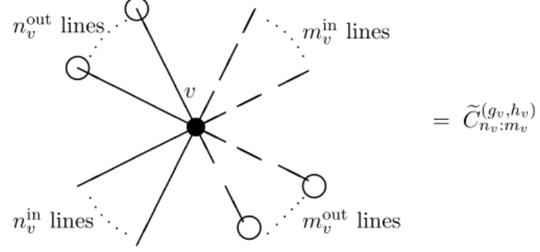
In other words, Li,v is the number of self-loops attached to the vertex v whose edges are of the type Eiin. Define non-negative integers ninv,noutv ,minv and moutv by
ninv = #{e∈E2in|v∈j2in(e)}+ #{e∈E1in|j1in(e) = (v,∗)}+ #L2,v+ #L1,v,
minv = #{e∈E0in|v∈j0in(e)}+ #{e∈E1in|j1in(e) = (∗, v)}+ #L0,v+ #L1,v,
noutv = #{e∈E1out |v∈j1out(e)}, moutv = #{e∈E0out |v∈j0out(e)}.
The valence val(v) of v ∈ V is given by val(v) = nv +mv, where nv := ninv +noutv (the number of solid lines attached tov),mv:=minv+moutv (the number of dashed lines attached to v). See Fig. 2.
Definition 3. (i) For a Feynman diagramG, define
(19) FG =
v∈V
C(gv,hv)
nv:mv ·
e∈Ein 0
(−2S)· e∈Ein
1
(−Sz)· e∈Ein
2
(−Szz)· e∈E0out
∆· e∈E1out
∆z.
(ii) Let Aut(G) be the automorphism group ofG. Define the groupAG by
AG=
e∈L0⊔L2
Z/2Z ⋉Aut(G),
i.e. AG fits into the following exact sequence:
1→(Z/2Z)#L0+#L2 →A
G→Aut(G)→1. This means that each self-loop of type Ein
0 and E2in contributes the factor 2 to #AG.
Definition 4. Let G(g, h) be the set of (isomorphism classes of) Feynman diagrams G
which satisfy the following conditions. (i) Gis connected.
(ii) For any v∈V, C(gv,hv)
nv:mv = 0.
(iii) Gsatisfies v∈V gv + #Ein−#V + 1 =g andv∈V hv+ #Eout=h. (iv) For any v∈V, val(v)>0.
Note that the set G(g, h) is a finite set. Note also that the graph whose amplitude is
F(g,h), i.e. the graph with only one vertex with label (g, h) and without edges is not a
(i)
e
✉
v1
✉
v2
=−2S
(ii)
e
✉
v1
✉
v2
=−Sz
(iii)
e
✉
v1
✉
v2
=−Szz
(iv)
e
✉
v ❤
= ∆
(v)
e
✉
v ❤
= ∆z
Figure 1. Three types of inner edges and propagators: (i) e ∈ E0in,
j0in(e) = {v1, v2}, (ii) e ∈ E1in, j1in(e) = (v1, v2), (iii) e ∈ E2in, j2in(e) =
{v1, v2}. Two types of outer edges and terminators: (iv) e ∈ E0out,
j0out(e) =v, (v) e∈E1out,j1out(e) =v.
v
① ✁ ✁ ✁ ✁ ✁ ✁
✟ ✟ ✟ ✟ ✟ ✟
nout
v lines
❥
❍ ❍ ❍ ❍ ❍ ❍
❥
❆ ❆ ❆ ❆ ❆ ❆
ninv lines
❆ ❆
❆ ❆ ❍❍
❍❍ ❍❍ ✟✟ ✟✟
✟✟
✁✁ ✁✁
✁✁
❥
❥
minv lines
moutv lines
= C(gv,hv)
nv:mv
Figure 2. A vertex v labeled by (gv, hv) to which nv = ninv +noutv solid
lines andmv=minv +moutv dashed lines are attached and its value.
Define
(20) FFD(g,h):=− G∈G(g,h)
1 #AG
FG.
The next result follows from [5].
Proposition 5. ∂¯zFFD(g,h)=the RHS of (8).
Therefore, the general solution F(g,h) of Walcher’s holomorphic anomaly equation is of
the form
(21) F(g,h)=FFD(g,h)+f(g,h),
wheref(g,h)is the holomorphic ambiguity which can not be determined from the equation
2.5. Holomorphic ambiguity. Recall that the holomorphic ambiguity f(g,0) (g≥2) is of the form [2][20, (2.30)]
f(g,0) = a0+a1z+· · ·+a2g−1z
2g−1
(1−55z)2g−2 + ⌊2g−2
5 ⌋
i=0
zj
for the closed sectorh= 0. Huang–Klemm–Quackenbush [13] determined the holomorphic ambiguity up to g ≤51 by using the vanishing of the BPS numbersngd (cf. footnote 4), the gap condition at the conifold pointz= 515 and the regularity condition at the orbifold
point z=∞.
For h >0, we assume that F(g,h) has poles of order at most 2g−2 +h at z = 1 55 and
also that the asymptotic behaviour at z=∞ isF(g,h) ∼z2g−2+h
2 [19, §3.3]. Therefore we
put the following ansatz for f(g,h):
f(g,h)=
a0+a1z+· · ·+a3g−3+3h 2 z
3g−3+3h 2
(1−55z)2g−2+h (h even),
f(g,h)= √
z(a0+a1z+· · ·+a3g−3+3h−1 2 z
3g−3+3h−1
2 )
(1−55z)2g−2+h (h odd). (22)
3. Polynomiality and PDE’s for F(g,h)
In this section, we consider extending Yamaguchi–Yau’s and Hosono–Konishi’s results [20, 12] toF(g,h).
3.1. The generators of polynomial ring. Letθz =z∂z∂ . We define
Ap =
θzGzz¯
Gzz¯
, Bp =
θze−K
e−K (p= 1,2, . . .) ,
Qp=z
1
2θzT (p= 0,1,2, . . .) ,
R1 =z
5 2e
KC zzz
Gzz¯
D¯zT , R2=z
7
2eKCzzzT.
(23)
The generators Ap’s and Bp’s were defined in [20]. The new ingredients are Qp’s, R1
and R2 which are necessary for incorporating△zz.
Consider the polynomial ring
(24) I =C(z)[A1, B1, B2, B3, Q0, Q1, Q2, Q3, R1, R2]
with coefficients in the field of rational functionsC(z).
Lemma 6. 1. Ap ∈I (p≥2), Bp ∈I (p≥4), Qp ∈I (p≥4).
Proof. First, notice that the logarithmic derivationθz acts as follows:
θzAp =Ap+1−ApA1 , θzBp =Bp+1−BpB1 ,
θzQp = 1
2Qp+Qp+1 ,
θzR1 = 5
2 −A1−B1+
θzCzzz
Czzz
R1+R2,
θzR2 = 7
2 −B1+
θzCzzz
Czzz
R2 .
(25)
Next we show A2, B4, Q4 ∈I. By the special geometry relation (1), we have
(26) A2 =−2A1B1+ 2B12+ 2B1−4B2+
θz(zCzzz)
zCzzz
(1 +A1+ 2B1) +h(z) .
Here h(z) is determined by comparing the behaviour of the RHS and the LHS at z= 0:
h(z) = 1−3·5
4z
1−55z .
Let us write the Picard–Fuchs operator asD=4p=0Hp(z)θzp whereHp(z)∈C[z]. Since De−K = 0,B
4 satisfies
(27) B4=−
3
p=1
Hp(z)
H4(z)
Bp−
H0(z)
H4(z)
= 0 .
Moreover, since T satisfies (3),
(28) Q4 =−
3
p=0
Hp(z)
H4(z)
Qp+ 60 24z.
These together with (25) implies thatI is closed with respect to the logarithmic deriva-tion θz. Moreover, by applyingθz recursively, we can show that Ap ∈I (p ≥3), Bp ∈ I
(p≥5),Qp ∈I (p≥5).
3.2. Polynomiality. For simplicity, we will use the notation
(29) V1=A1+ 2B1+ 1, V2 =B2−B1V1
from here on.
Since Dz acts on (TMcpl)
m⊗ Ln as
Dz = 1
z(θz+mA1+nB1) ,
we have the following
Lemma 7. Let f be a section of (TMcpl)
m⊗ Ln. Then D
zf ∈I iff ∈I and Dzf ∈√zI
if f ∈√zI.
Lemma 8. Fn(g,h)∈z
Proof. We prove the lemma by induction on (g, h).
For (g, h) = (0,0),(1,0),(0,1),(0,2), the lemma is true since
F3(0,0)=Czzz ∈I,
F1(1,0)=
1 2z
−A1−
62 3 B1−
31 6 −
1 6
θz(1−55z) (1−55z)
∈I,
F2(0,1)=△zz =z−
5
2[Q2−V1Q1−V2Q0−R1] ∈√z I,
F1(0,2)=
1△zz 2Czzz −
B1
2z +f
(0,2)
∈I.
(30)
For (g, h)= (0,0),(1,0),(0,1),(0,2), assume thatFn(g′,h′)∈z
h
2Iholds for every (g′, h′)=
(g, h) such thatg′ ≤gandh′ ≤h. Consider the contributionF
Gfrom a Feynman diagram
G∈G(g, h) to F(g,h)
FD (19). The assumption of the induction implies that a vertex factor
satisfies C(gv,hv)
nv;mv ∈z hv
2 I. As for edge factors, the followings hold. From (10),
Szz = 1
zCzzz
−A1−2B1−8
5
∈I, Sz= 1
z2C
zzz
B2+ 3B1+ 2
25
∈I.
(31)
By Lemma 7,S also satisfies S ∈I. Similarly by (30) the terminators (11) satisfy
△z,△ ∈√zI.
Therefore, by the condition (iii) in Definition 4, we haveFG ∈z
h
2I and thusF(g,h)
FD ∈z
h 2I.
As to the holomorphic ambiguity f(g,h), it satisfiesf(g,h)∈zh2C(z)⊂z h
2 I by assumption
(22). ThereforeF(g,h)∈I. Forn≥1,F(g,h)
n ∈I by Lemma 7.
Definition 9. Let g, h, n≥0 be integers satisfying 2g−2 +h+n >0. We define
(32) Pn(g,h)= (z3Czzz)g+h−1zh2F(g,h)
n , P(g,h):=P
(g,n)
0 .
For other values of (g, h, n), we setPn(g,h)= 0.
Lemma 8 implies that
Pn(g,h) ∈ I.
Remark 10. Letx=z3C
zzz = 1−555z. Consider the graded ring
C[x, A1, B1, B2, B3, Q0, . . . , Q3, R1, R2],
where the grading is given by deg x= 1, degA1 = 1, degBp =p (p= 1,2,3), degQp =p (p= 0,1,2,3), degR1= 2 and degR2= 3. ThenP(g,h) belongs to this ring and its degree
is at most 3(g+h−1).
Lemma 11.
∂¯zB2 =V1∂¯zB1 ,
∂¯zB3 = (A2+ 2A1+ 3B1+ 3B2+ 3A1B1+ 1)∂z¯B1
=−V2+
θz(z3Czzz)
z3Czzz V1+h(z)−1
∂¯zB1
∂z¯Qp = 0 (p= 0,1,2, . . .) ,
∂¯zR2 =−R1∂z¯B1 .
(33)
Proof. The first and the second equations were obtained from (1) in [20]. The third is
trivial since Qp’s do not depend on ¯z. The calculation of ∂¯zR2 is as follows.
∂z¯R2 =zα+1Czzz(∂z¯T¯+∂z¯K·T¯) =zGzz¯R1 =−R1∂z¯B1
where we have used the identityGz¯z=∂z∂z¯K(z,z¯) =−∂z¯B1/z.
If one assumes that ∂z¯A1, ∂z¯B1, ∂z¯R1 are independent, the Walcher’s extended
holo-morphic equation (8) is rewritten as follows.
Lemma 12. The equation(8) is equivalent to the system of PDE’s:
−R1
∂ ∂R2 −
2 ∂
∂A1
+ ∂
∂B1
+V1
∂ ∂B2
(34)
+−V2+
θz(z3Czzz)
z3C
zzz
V1+h(z)−1
∂
∂B3
P(g,h)= 0 ,
∂P(g,h)
∂A1
=−1 2
g1+g2=g,
h1+h2=h
P(g1,h1)
1 P
(g2,h2)
1 +P
(g−1,h) 2
+ (B1Q0−Q1)P1(g,h−1) ,
(35)
∂P(g,h)
∂R1
=−P1(g,h−1) .
(36)
Here the summation in (35) runs over (g1, h1),(g2, h2) such that(gi, hi)= (0,0),(0,1).
Proof. By (8), we have
∂z¯P(g,h)=
1
2∂¯z(zCzzzS zz)
·
g1+g2=g,
h1+h2=h
P(g1,h1)
1 P
(g2,h2)
1 +P
(g−1,h) 2
−∂z(¯ z
5
2Czzz△z)·P(g,h−1)
1 .
Note that, by (31)(33),
∂¯z(zCzzzSzz) =−(∂¯zA1+ 2∂z¯B1),
∂¯z(z
5
2Czzz△z) =−(∂¯zA1+ 2∂z¯B1)(−Q1+B1Q0) +∂¯zR1 .
On the other hand, by (33), ∂z¯ in the LHS is as follows :
∂z¯=∂z¯R1
∂ ∂R1
+∂z¯A1
∂ ∂A1
+∂z¯B1
−R1
∂ ∂R2
+ ∂
∂B1
+V1
∂ ∂B2
+−V2+
θz(z3Czzz)
z3C
zzz
V1+h(z)−1
∂
∂B3
Inserting these and comparing the coefficients of ∂z¯A1, ∂z¯B1, ∂z¯R1, one obtains Lemma
12.
To write the equations in a more useful form, we change the generators. We define
u=B1, v1=V1+
3
5, v2 =V2+ 2 25,
v3 =B3−B1
−V2+
θz(z3Czzz)
z3C
zzz
V1+h(z)−1
+s(z),
m1=
2 25Q0+
3
5Q1+Q2−R1,
m2=Q0
s(z)− 2 25
θz(z3Czzz)
z3C
zzz
+Q1 23
25−h(z)
−Q2
θz(z3Czzz)
z3C
zzz +Q3−R2−B1R1,
(37)
where
(38) s(z) = 12 25 −
1 5h(z) +
3 25
θz(z3Czzz)
z3C
zzz
.
Define the ring
J :=C(z)[u, v1, v2, v3, Q0, Q1, Q2, Q3, m1, m2].
It is isomorphic to I since (37) is invertible. Notice that θz :J → J increases the degree inu at most by 1.
Now we regard P(g,h) ∈ J. Then (34) implies P(g,h) is independent of u. In turn,
Pn(g,h) ∈J has degree at most nin u. Following [12, (3-4.c)], let us define u-independent polynomialsY0, Y1, W0, W1, W2 ∈J by
Y0+u Y1 =P1(g,h−1),
W0+uW1+u2W2= (the RHS of (35)).
(39)
Then applying the change of generators (37) to the equations (34)(35)(36), we obtain
Theorem 13. The equation(8)is equivalent to the following system of PDE’s forP(g,h)∈ J :
∂ ∂uP
(g,h)= 0,
∂ ∂m1
P(g,h)=Y0,
∂ ∂m2
P(g,h)=Y1,
∂ ∂v1
P(g,h)=W0,
∂ ∂v2
P(g,h)=−W1+
θz(z3Czzz)
z3C
zzz
W2,
∂ ∂v3
P(g,h)=−W2.
(40)
Let us comment on the constant of integration. Decompose P(g,h) as
P(g,h)= ˆP(g,h)+P(g,h)|v1,v2,v3,m1,m2=0
where ˆP(g,h)consists of terms of degree≥1 with respect to at least one ofv
1, v2, v3, m1, m2.
a polynomial in Q0, Q1, Q2, Q3 with C(z) coefficients. However, the choice of the new
generators (37) is “good” (cf. [12, (3-4.d)]) so that we have the following
Proposition 14.
P(g,h)|v1,v2,v3,m1,m2=0= (z
3Czzz)g+h−1zh 2f(g,h).
Proof. We have
Szz =− v1
zCzzz
, Sz = uv1+v2
z2Czzz ,
S = 1
z3C
− 12u2v1−
u+ 5
5z
2(1−55z)
v2+
v3
2
,
△z = 1
z52Czzz
(−m1+Q1v1+Q0v2),
△= 1
z72Czzz
um1−m2−uQ0v1−v2
uQ0+
55z
1−55zQ0+Q1
+Q0v3
.
Notice that every monomial term in the propagatorsSzz, Sz, S and the terminators△z,△ contains at least one of v1, v2, v3, m1, m2. Therefore the Feynman diagram part FF D(g,h) of F(g,h) has degree at least one with respect to one of v1, v2, v3, m1, m2 by (19)(20). This
implies that the first term in the RHS of
P(g,h)= (z3Czzz)g+h−1z
h 2F(g,h)
F D + (z3Czzz)g+h−1z
h 2f(g,h)
vanishes as v1, v2, v3, m1, m2 go to zero. This proves the proposition.
4. Fixing holomorphic ambiguity and n(dg,h)
Let ω0(z),ω1(z), ω2(z), ω3(z) be the following solutions to the Picard–Fuchs equation
Dω = 0 aboutz= 0.
ωi(z) =∂ρi
n≥0
(5ρ+ 1)5n (ρ+ 1)n5 z
n+ρ
ρ=0
.
Let t =ω1(z)/ω0(z) be the mirror map and consider the inverse z =z(q) whereq = et.
Explicitly, these are
ω0(z) = 1 + 120z+ 113400z2+· · · ,
ω1(z) =ω0(z) logz+ 770z+ 810225z2+· · · ,
t= 770z+ 717825z2 +3225308000 3 z
3+
· · ·, z=q−770q2+ 171525q3 +· · · .
Let
(41) FA(g,h) = lim
¯
z→0F (g,h)ω
for (g, h) satisfying 2g+h−2>0 6. The limit ¯z→0 in the RHS means
Gzz¯→
dt
dz, e
K
→ω0(z), △zz →DzDzT.
Define n(dg,h) forh >07 by the formula [15] [14] [19, (3.22)]:
the terms in positive powers in q of
∞
g=0
gs2g+h−2FA(g,h)
=
∞
g=0
d
k
n(dg,h)1 k
2 sinkgs 2
2g+h−2
qkd2 .
(42)
Here the summation of k is over positive odd integers and that of dis over positive even (resp. odd) integers when h is even (resp. odd).
Remark 15. It is expected that FA(g,h) is the A-model topological string amplitude of genus g with h boundaries for the real quintic 3-fold (X, L), and that n(dg,h) be the BPS invariants in the classd∈H2(X, L;Z). See [7, 21] for (g, h) = (0,0),(1,0) and [18, 16] for
(g, h) = (0,1).
In order to fix the holomorphic ambiguity, we put the following assumptions.
(i) Ifh is even, the q-constant term in FA(g,h) vanishes except for (g, h) = (0,2). (ii) n(dg,h)= 0 ford≤d0whered0is the smallest number necessary to completely
deter-mine unknown parameters inf(g,h). For example,d
0 = 3 for (g, h) = (0,3),(1,1),
d0 = 6 for (g, h) = (1,2),(0,4) and d0 = 9 for (g, h) = (1,3),(0,5).
The numbers n(dg,h) obtained under these assumptions are listed in Tables 1 and 2.
Remark 16. The boundary conditions proposed in [19] are the condition (i) and the con-dition that
(43) n(dg,h)= 0 if n2dg+h−1 = 0.
These do not give enough equations to fix the unknown parameters off(g,h), unless (g, h) =
(0,1),(0,2),(0,3),(1,1). For this reason we assumed (ii) instead of (43).
Remark17. For the cases listed in Tables 1 and 2,n(dg,h)turn out to be integers. However,
for (g, h) = (0,7),(1,5),(2,1), the holomorphic ambiguities determined by our assump-tions do not give integraln(dg,h)’s.
6For (g, h) = (0,0),(1,0),(0,1),(0,2), one should consider
∂tnF (g,h) A =
“dz
dt
”n lim ¯ z→0F
(g,h) n ω2
g+h−2
0
wheren= 3,1,2,1, respectively.
7Forh= 0, the BPS numberng
dis defined by [8]
∞ X
g=0 gs2g
−2
FA(g,0)=
∞ X
g=0
X
d>0
X
k>0 ngd1
k
“
2 sinkgs 2
”2g−2
d n(0d,4)
2 0
4 0
6 0
8 −307669500
10 −1290543544800 12 −4192442370526500 14 −11974312128284645400 16 −31709386561589633978460 18 −79870219101822591783739800 20 −194146223749422074623095454800
d n(0d,5)
1 0
3 0
5 0
7 0
9 0
11 −101052180000 13 −6448499064000 15 2809704427965432000 17 19034205058652662269000 19 85987169904148441092385200
d n(0d,6)
2 0
4 0
6 0
8 0
10 0
12 0
14 10969992383850000 16 88807052603386080000 18 453871851092663617206000 20 1856308715086126538509560000
Table 1. n(dg,h) for (g, h) = (0,4),(0,5),(0,6)
Remark 18. As a final remark, let us comment on the expansion about the conifold point
z = 515. By expanding F(0,4) about z = 515, we see that there is no gap condition such as
the one found in [13, (1.2)]. On the other hand, if one imposes the gap condition toF(0,4)
instead ofn(06,4) = 0, then the integrality ofn(0d,4)’s does not hold.
Appendix A. Examples of Feynman diagrams
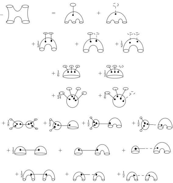
Feynman diagrams for FFD(0,3) and FFD(1,1) have been given in eqs. (2.109) and (2.108) of [19] respectively (#G(0,3) = #G(1,1) = 4). For (g, h) = (0,4), we have #G(0,4) = 19.
See Fig. 3. It is clear that the number of Feynman diagrams grows rapidly as g and h
d n(1d,1)
1 0
3 0
5 −222535
7 −472460880
9 −970639017980 11 −1925950714205525 13 −3771152449472734885 15 −7341083828377813532445 17 −14254813486499789264497980 19 −27655486644196368361422400900
d n(1d,2)
2 0
4 0
6 0
8 −1798092240
10 −3910898328975 12 −3254492224834500 14 11749281716111889000 16 75858033724596666836250 18 284100639663878543462155290 20 881568399267730913608111758000
d n(1d,3)
1 0 3 0 5 0 7 0 9 0 11 59476704611850 13 376498723243912410 15 1597793312432171312570 17 5622302692504776557418000 19 17697465511801448466779111250
d n(1d,4)
2 0 4 0 6 0 8 0 10 0 12 0
14 −510835096894879500 16 −4625213168889849497100 18 −26075494174267321098602160 20 −116382815077174964736448167150 Table 2. n(dg,h) for (g, h) = (1,1),(1,2),(1,3),(1,4)
Appendix B. f(0,4) and P(0,4)
f(0,4)= 2−20125z+ 70618750z
2 −86493078125z3
10000 (1−3125z)2 .
P(0,4)
=z 2(
−2 + 20125z−70618750z2+ 86493078125z3)
80 (−1 + 3125z)5
−
z(2−9500z+ 16015625z2)m12 20 (−1 + 3125z)3
+(−9 + 12500z)m1 4
120 (−1 + 3125z)
+75z 2(
−1 + 3145z)m2 4 (−1 + 3125z)3
+m1 3m
2 6 +
5z m22 4 (−1 + 3125z)
+m1( 375z3(
−3 + 3125z)
2 (−1 + 3125z)4
+ 375z 2m
2 2 (−1 + 3125z)2
)− Q14v15
8 + (
(−3 + 25000z)Q04 40 (−1 + 3125z) −
Q03Q1 6 )v2
4
+v14(
m1Q13 2 +
(−9 + 12500z)Q14 120 (−1 + 3125z)
−
Q0Q13v2 2 ) + (
25z2
8 (−1 + 3125z)2 −
75z2(−1 + 3145z)Q0 4 (−1 + 3125z)3
−
375z2m 1Q0 2 (−1 + 3125z)2
− m13Q0
6 −
5z m2Q0 2 (−1 + 3125z)
)v3+
5z Q02v32 4 (−1 + 3125z)
+v22(
z(−1 + 4750z+ 119921875z2)Q02 10 (−1 + 3125z)3
+m1( − 5z Q0 2 (−1 + 3125z)
+m2Q0 2
2 )
−
8000z2Q0Q1 (−1 + 3125z)2
+ 5z Q1 2
4 (−1 + 3125z)
+m12(
(−9 + 43750z)Q02 20 (−1 + 3125z)
− Q0Q1
2 )−
− = +
+ 12 + + 12
+ 16 + 12
+ 241 + 16
+ 18 + 12 + 12 + 12
+ 12 + +
+ 12 + + 12
Figure 3. The elements G inG(0,4) and the orders of AG. The vertices
are expressed as bordered Riemann surfaces to visualize the labeling.
+v23(
5z Q02 4 (−1 + 3125z)
− m2Q03
6 +m1(
−((−9 + 59375z)Q03) 30 (−1 + 3125z)
+Q0 2Q
1 2 ) +
Q04v3 6 )
+v13( − 375z2Q
12 4 (−1 + 3125z)2
−
3m12Q12 4 −
(−9 + 12500z)m1Q13 30 (−1 + 3125z)
− m2Q13
6
+ (3m1Q0Q1 2
2 +
3Q0Q13 10 −
Q14 6 )v2−
3Q02Q12v22
4 +
Q0Q13v3 6 )
+v2(
81875z3
8 (−1 + 3125z)3 −
236625z3Q0 4 (−1 + 3125z)3
+m12( 5z
4 (−1 + 3125z) −
m2Q0 2 )
+m13(− 3Q0 10 +
Q1 6 ) +
75z2(−1 + 3145z)Q1 4 (−1 + 3125z)3
+m1(
z(−1 + 1625z)Q0 5 (−1 + 3125z)2
+ 375z 2Q
1 2 (−1 + 3125z)2
)
+m2( −
8000z2Q0 (−1 + 3125z)2
+ 5z Q1 2 (−1 + 3125z)
) + ( 8000z 2Q
02 (−1 + 3125z)2
+m1 2Q
02 2 −
5z Q0Q1 2 (−1 + 3125z)
)v3)
+v1( − 140625z4
8 (−1 + 3125z)4 −
m14 8 −
375z3(−3 + 3125z)Q1 2 (−1 + 3125z)4
+z(2−9500z+ 16015625z
2 )m1Q1 10 (−1 + 3125z)3
−
(−9 + 12500z)m13Q1 30 (−1 + 3125z)
−
375z2m2Q1 2 (−1 + 3125z)2
+m12( − 375z2
4 (−1 + 3125z)2 −
m2Q1 2 )
+ (m1Q0 3
2 +
(−9 + 59375z)Q03Q1 30 (−1 + 3125z)
− Q02Q12
2 )v2 3
− Q04v24
8
+ ( 375z 2Q
0Q1 2 (−1 + 3125z)2
+m1 2Q
0Q1
2 )v3+v2(
m13Q0 2 −
z(−1 + 1625z)Q0Q1 5 (−1 + 3125z)2
−
+m1(
375z2Q0 2 (−1 + 3125z)2
−
5z Q1 2 (−1 + 3125z)
+m2Q0Q1) +m12( 9Q0Q1
10 −
Q12
2 )−m1Q0 2Q
1v3)
+v22( − 375z2Q
02 4 (−1 + 3125z)2
−
3m12Q02 4 +
5z Q0Q1 2 (−1 + 3125z)
−
m2Q02Q1 2
+m1(−
((−9 + 43750z)Q02Q1) 10 (−1 + 3125z)
+Q0Q12) +
Q03Q1v3 2 ))
+v12(
m13Q1 2 −
z(2−9500z+ 16015625z
2 )Q12 20 (−1 + 3125z)3
+(−9 + 12500z)m12Q12 20 (−1 + 3125z)
+m1(
375z2Q1 2 (−1 + 3125z)2
+m2Q1 2
2 ) + (
3m1Q02Q1
2 +
(−9 + 43750z)Q02Q12 20 (−1 + 3125z)
− Q0Q13
2 )v2 2
−
Q03Q1v23
2 −
m1Q0Q12v3 2 +v2(
−375z
2Q 0Q1 2 (−1 + 3125z)2
−
3m12Q0Q1
2 +
5z Q12 4 (−1 + 3125z)
−
m2Q0Q12 2 +m1(
−9Q0Q12 10 +
Q13 2 ) +
Q02Q12v3 2 )).
References
[1] Murad Alim and Jean Dominique L¨ange,Polynomial Structure of the (Open) Topological String Par-tition Function, arXiv:0708.2886 [hep-th].
[2] M. Bershadsky, S. Cecotti, H. Ooguri, C. Vafa,Kodaira-Spencer Theory of Gravity and Exact Results for Quantum String Amplitudes, Commun.Math.Phys.165(1994) 311-428, [hep-th/9309140].
[3] G. Bonelli and A. Tanzini,The holomorphic anomaly for open string moduli, arXiv:0708.2627 [hep-th]. [4] Philip Candelas, Xenia C. de la Ossa, Paul S. Green and Linda Parkes,A pair of Calabi-Yau manifolds
as an exactly soluble superconformal theory, Nuclear Phys.B359(1991), 21–74.
[5] Paul L. H. Cook, Hirosi Ooguri and Jie Yang, Comments on the Holomorphic Anomaly in Open Topological String Theory, arXiv:0706.0511 [hep-th].
[6] Hao Fang, Zhiqin Lu and Ken-Ichi Yoshikawa, Analytic torsion for Calabi-Yau threefolds, arXiv:math/0601411.
[7] Alexander B. Givental, Equivariant Gromov-Witten invariants, Internat. Math. Res. Notices 1996, no. 13, 613–663.
[8] R. Gopakumar and C. Vafa,M-theory and topological strings. I, II, th/9809187, arXiv:hep-th/9812127.
[9] Mark L.Green,Infinitesimal methods in Hodge theory, In Algebraic cycles and Hodge theory (Torino, 1993), 1–92, Lecture Notes in Math.1594, Springer, Berlin, 1994.
[10] B.R. Greene and M.R.Plesser, Duality in Calabi-Yau moduli space, Nuclear Phys.B 338 (1990), no.
1, 15–37.
[11] Phillip Griffiths ed., Topics in transcendental algebraic geometry, Proceedings of a seminar held at the Institute for Advanced Study, Princeton, N.J., during the academic year 1981/1982, Annals of Mathematics Studies106, Princeton University Press, Princeton, NJ, 1984.
[12] Shinobu Hosono and Yukiko Konishi, Higher genus Gromov-Witten invariants of the Grassmannian, and the Pfaffian Calabi-Yau threefolds, arXiv:0704.2928 [math.AG].
[13] Min-xin Huang, Albrecht Klemm, Seth Quackenbush,Topological String Theory on Compact Calabi-Yau: Modularity and Boundary Conditions, arXiv:hep-th/0612125.
[14] J. M. F. Labastida, M. Marino and C. Vafa, Knots, links and branes at large N, JHEP 0011, 007
(2000) [arXiv:hep-th/0010102].
[15] H. Ooguri and C. Vafa, Knot invariants and topological strings, Nucl. Phys. B577(2000), 419–438
[arXiv:hep-th/9912123].
[16] R. Pandharipande, J. Solomon, J. Walcher, Disk enumeration on the quintic 3-fold, arXiv:math/0610901.
[18] Johannes Walcher, Opening mirror symmetry on the quintic, arXiv:hep-th/0605162, To appear in Commun. Math. Phys..
[19] , Extended holomorphic anomaly and loop amplitudes in open topological string, arXiv:0705.4098 [hep-th].
[20] Satoshi Yamaguchi and Shing-Tung Yau,Topological String Partition Functions as Polynomials, JHEP 0407 (2004) 047, [arXiv:hep-th/0406078].
[21] Aleksey Zinger, The Reduced Genus-One Gromov-Witten Invariants of Calabi-Yau Hypersurfaces, arXiv:0705.2397[math.AG]
Graduate School of Mathematical Sciences, The University of Tokyo, 3-8-1 Komaba,
Meguro, Tokyo 153-8914 Japan
E-mail address: [email protected]
Department of Mathematics, Hokkaido University, Kita 10, Nishi 8, Kita-Ku, Sapporo
060-0810, Japan