虚数化学ポテンシャル法に基づくQCD相図の研究
管野, 淳平
https://doi.org/10.15017/1931695
出版情報:Kyushu University, 2017, 博士(理学), 課程博士 バージョン:
権利関係:
Approach to QCD phase diagram based on the imaginary chemical
potential method
Junpei Sugano
Theoretical Nuclear Physics, Department of Physics
Graduate School of Science, Kyushu University
744, Motooka, Nishi-ku, Fukuoka 819-0395, Japan
Abstract
Matters in our world are composed of the quarks that interact with each other through the strong interaction mediated by gluons. The Quantum Chromodynamics (QCD) is the non-abelian gauge theory that describes the dynamics of quarks and gluons. One of remarkable properties of the QCD is asymptotic freedom, which makes coupling constant of the strong inter- action decrease as increasing the energy scale and vice versa. In virtue of the asymptotic freedom, it is expected that the quark-gluon system takes various states, in response to the change of external parameters. It is chal- lenging and interesting in hadron physics to clarify properties of the QCD under various external parameters, which leads to understanding of the early universe, neutron star physics and so on. In particular, toward understand- ing of the inner structure of neutron star, it is essential to study the QCD and its phase diagram under finite light-quark chemical potential µl, isospin chemical potential µiso, and strange-quark chemical potential µs.
Among the theoretical approaches, lattice QCD (LQCD) simulations are the most reliable framework, since it is the first-principle calculation of the QCD. LQCD simulation, however, suffers from the sign problem and thereby the simulation is difficult to work. It is thus important to gather solid infor- mation from the regions where the sign problem does not occur.
In this thesis, we focus on the following three imaginary chemical potential regions; (A) the imaginary µl region, (B) the imaginaryµl andµs region, (C) the imaginary µl and µiso region. In these regions, LQCD simulations can be performed since there is no sign problem. Information on real µl, µiso, µs regions is extracted by the analytic continuation from the imaginary region to the real one. We call this procedure “imaginary chemical potential method”.
It is thus important to know the analyticity of the QCD in order to apply the imaginary chemical potential method.
For region (A), the phase structure of the QCD has been investigated in detail, and it was found that the first-order Roberge-Weiss phase transition prevents the analytic continuation. Due to this, information on the real-µl dependence of physical quantities is limited up to µl/T ≲ 1, where T is temperature. To analyze the region µl/T ≳ 1, it is convenient to use the effective models that are consistent with LQCD data in µl/T ≲ 1. Our purpose in region (A) is to construct a reliable effective model to describe the quark degree of freedom. We aim at determining the strength of the
i
we analyze the QCD phase diagram and the inner core of neutron star.
As for region (B) and (C), there are little studies and it is therefore desirable to explore properties of the QCD there. In region (B), we take two approaches; one is a theoretical approach based on the QCD and the other is a model approach with the same properties as the QCD as possible.
The latter is a qualitative approach, but it allows us flexible investigation.
In region (A), the analyticity is lost by the presence of the first-order phase transition. We thus study the location of the first-order transition in region (B). Furthermore, we search the condition imposed on imaginary µl and µs, in order to obtain the region where no first-order transition takes place. If such a region exists, it is useful for the imaginary chemical potential method.
In the real µiso region, the QCD has a characteristic phase, called the charged-pion condensate phase. In the phase, flavor UI3(1) symmetry of the QCD is spontaneously broken and the sign problem is expected to be severe.
This means that LQCD simulations become unfeasible there. Meanwhile, it is predicted that the charged-pion condensate does not occur in the imaginary µiso, at least forµl = 0. We show that this prediction is true also for non-zero µl, i.e., in region (C). For the proof, we use QCD inequalities. This approach enables us to see which symmetry is spontaneously broken or not, based on the QCD. The proof is done by demonstrating that UI3(1) symmetry is not spontaneously broken in region (C).
This thesis is based on the following three papers:
• Determination of hadron-quark phase transition line from lattice QCD and two-solar-mass neutron star observations,
J. Sugano, H. Kouno, and M. Yahiro, Phys. Rev. D94, 014024 (2016).
• Properties of 2+1-flavor QCD in the imaginary chemical potential re- gion: A model approach,
J. Sugano, H. Kouno, and M. Yahiro, Phys. Rev. D96, 014028 (2017).
• QCD-inequality analyses on pion condensate at real and imaginary isospin chemical potentials under finite imaginary quark chemical po- tential,
J.Sugano, H. Kouno, and M. Yahiro, arXiv:1711.00663 (to be published in Physical Review D).
Acknowledgements
First of all, I would like to express my sincere gratitude to my supervisor Prof. Masanobu Yahiro. The discussions with him were exciting for me and I learned many knowledge on hadron physics, particle physics, and astro- physics. He also showed me attitude as researcher and educator. In addi- tion, he always supported and encouraged me on my research since I was undergraduate student. Thanks to him, I accomplished my Dr. thesis.
I would like to express appreciation to Prof. Hiroaki Kouno. He gave me many comments and insights on hadron physics. His comments allowed me to grasp the essence and intuitive understanding of hadron physics. He also taught me rigor of research.
I would like to express my appreciation to Associate Prof. Yoshifumi R.
Shimizu and Assistant Prof. Takuma Matsumoto. Through their seminar, I could learn how nuclear structure and reaction, and quantum field theory are interest and difficult. Moreover, they gave me many comments in the view point of nuclear physicist.
I was supported by many seniors and juniors of theoretical nuclear physics laboratory and would like to express my gratitude to them. I especially would like to thank to six seniors. First, I would like to appreciate to two seniors, Dr.
Kouji Kashiwa and Dr. Junichi Takahashi. They gave me warm words and valuable comments on research. Next, I would like to express my appreciation to four seniors, Dr. Shin Watanabe, Dr. Masahiro Ishii, Dr. Satoru Sasabe, and Dr. Masakazu Toyokawa. They were always open and taught me many knowledges on hadron physics, nuclear physics, and computational technique in casual conversation. Furthermore, I did enjoy private life with them.
I would like to extend my appreciation to people of other laboratories.
In particular, I would like to express my special thanks to Aya Kasai. She taught me many ideas on particle physics and I was always encouraged by her warm words.
I would like to show my appreciation to Yuki Yamaji, Hiromi Tsuchi- jima, Megumi Ieda, Noriko Taguchi, Mayumi Takaki, and Mariko Komori for practical supports to me and amusing conversation.
This work was supported by Grants-in-Aid for Scientific Research (No.
27-7804) from the Japan Society for the Promotion of Science (JSPS).
Finally, I would like to express my deepest appreciation to my family: my parents and sisters. They always encouraged me through all my life.
iii
acknowledgements iii
1 Introduction 1
1.1 QCD in Minkowski space-time . . . 1
1.2 QCD phase diagram . . . 3
1.3 Lattice QCD . . . 9
1.4 Imaginary chemical potential method . . . 11
1.5 Purpose . . . 15
2 Hadron-quark phase transition line 16 2.1 Introduction . . . 16
2.2 EPNJL model with vector-type interaction . . . 17
2.3 Relativistic mean field theory . . . 21
2.4 Two phase model . . . 25
2.5 Phase transition line without Gv. . . 26
2.6 Effects of Gv on hadron-quark transition line . . . 27
2.7 Density dependence ofGv . . . 28
2.8 Short summary . . . 30
3 2+1-flavor QCD in the imaginary region 32 3.1 Introduction . . . 32
3.2 RW periodicity in the QCD . . . 32
3.3 2+1-flavor PNJL model . . . 34
3.4 Thermodynamic potential . . . 34
3.5 RW periodicity and its breaking in the PNJL model . . . 36
3.6 Numerical results . . . 36
3.7 Short summary . . . 41
4 QCD with isospin chemical potential 44 4.1 Introduction . . . 44
4.2 Fermion determinant and γ5-hermiticity . . . 45
4.3 QCD inequalities and charged-pion condensate . . . 48
4.4 Short summary . . . 50 iv
CONTENTS v
5 Summary 52
Appendix 55
A Notations in Euclidean space-time . . . 55 B Chiral transformation . . . 55 C Mean field approximation to the 2+1-flavor PNJL model . . . 57 D Some properties of physical quantity at finite θl . . . 58
action . . . 2
1.2 QCD phase diagram in T-µq plane . . . 8
1.3 Sketch of the link variable . . . 10
1.4 Phase diagram in T-θl plane in the 2-flavor QCD . . . 12
1.5 Phase diagram in T-θl plane in the 2+1-flavor QCD . . . 14
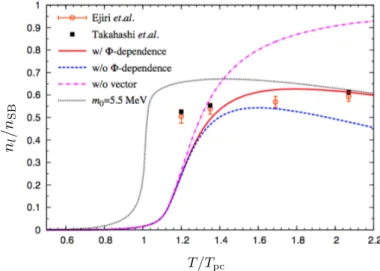
2.1 T dependence of nl . . . 21
2.2 Equation of state for symmetric and neutron matters . . . 24
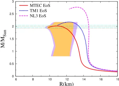
2.3 MR relation calculated from RMF theories . . . 25
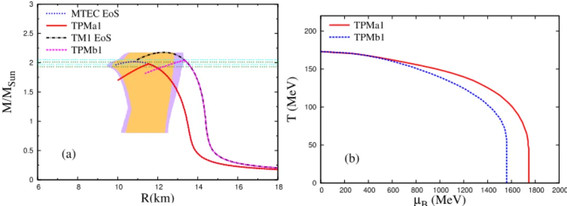
2.4 MR relation calculated by TPMa1 and TPMb1 . . . 27
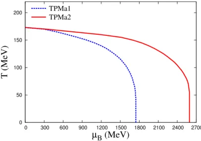
2.5 Hadron-quark phase transition line calculated by TPMa2 . . . 28
2.6 MR relation calculated from TPMa3 and TPMb3. . . 29
2.7 Band of the hadron-quark phase transition line . . . 30
3.1 Thermodynamic potential and quark number density for θl=θs 37 3.2 Thermodynamic potential and quark number density for θs = 0 37 3.3 QCD phase diagram for θl =θs . . . 39
3.4 QCD phase diagram for θs = 0 . . . 40
3.5 The θl dependence of the chiral transition line . . . 41
3.6 Analyticity of u-quark number density . . . 42
3.7 Analyticity of s-quark number density . . . 42
vi
List of Tables
1.1 Summary of the current-quark mass . . . 2 2.1 Summary of the parameter set in Polyakov-loop potential . . . 18 2.2 Summary of the parameter set in the 2-flavor EPNJL model . 19 2.3 Summary of the parameter set in the RMF theory . . . 23 2.4 Maximum mass and radius for the RMF parameter sets . . . . 25 2.5 The label of two-phase model . . . 26 2.6 The label of two-phase model with the density-dependent vector-
type interaction . . . 29 3.1 Summary of the parameter set in the 2+1-flavor PNJL model 36 3.2 Location of the RW-like transition point . . . 39 4.1 Positivity of the fermion determinant for real and imaginary
µiso . . . 47
vii
Chapter 1 Introduction
1.1 QCD in Minkowski space-time
The QCD in Minkowski space-time is constructed so that its Lagrangian is invariant under local gauge transformation, belonging to color SU(Nc) group, where Nc is the number of color. From any function U(x) ∈ SU(Nc), color SU(Nc) gauge transformation is defined by
q(x) → U(x)q(x),
Aµ(x) → U(x)Aµ(x)(U(x))−1+i(∂µU(x))(U(x))−1, (1.1) whereq = (q1,· · · , qNf) is the quark field with Nf flavors andAµ is the gluon field. The function U(x) is written as U(x) = exp(iθa(x)Ta) with any real functionθa(x), the generatorsTa, and color indicesa= 1,· · · , Nc2−1. In the gluon field, the notation Aµ =gAaµTa is used, i.e., the field Aµ includes the gauge coupling g in itself. Hereafter, we set Nc = 3. In this case, Ta=λa/2 with the Gell-Mann matrices λa.
Imposing the invariance under Eq. (1.1), the QCD Lagrangian is given by 1)
LQCD= ¯q(iγµDµ−m)qˆ − 1
2g2TrcFµνFµν. (1.2) In Eq. (1.2),Dµ =∂µ+iAµis the covariant derivative and ˆm = diag(m1,· · · , mNf) is the current quark-mass matrix in flavor space. The field strength of the gluon field is defined by
Fµν = 1
i [Dµ, Dν] =∂µAν −∂νAµ+i[Aµ, Aν]. (1.3) The symbol Trcin the right side of Eq. (1.2) denotes the trace in color space.
In experiments, six quarks have been confirmed so far, i.e., up (u), down (d), strange (s), charm (c), beauty (b), and top (t). The values of the current masses are tabulated in Table 1.1. The masses of c-, b-, and t-quarks are
1)We do not consider the so-calledθterm that violatesCP symmetry [1, 2, 3].
1
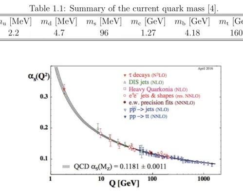
Figure 1.1: The energy scale Q dependence of the coupling constant αs(Q2) of strong interaction. The experimental data are presented with the error bars, and band means the theoretical prediction from the QCD. Figure is taken from [4].
much heavier than those of u-, d-, and s-quarks. In this thesis, we concentrate on the energy scale in which contributions of the heavy quarks can be ignored, and take into account only u-, d-, and s-quarks. Among these three quarks, u- and d-quarks have almost the same masses as each other, and hence we can set mu =md =ml as a good approximation. Under this approximation, we call the QCD with u- and d-quarks “2-flavor QCD”. Meanwhile, s-quark has a relatively large mass compared with u- and d-quarks, and consequently, the approximation ms =ml may not work well. Whenever we consider the QCD with the conditions of mu = md =ml and ms > ml, we call it “2+1-flavor QCD”.
One of the most important properties of the QCD is the asymptotic free- dom. Due to this property, the strength αs(Q2) of the quark-quark inter- action decreases as increasing the energy scale Q. The Q dependence can be calculated from the renormalization group equation. Up to the one-loop order, the result is given by [5, 6]
αs(Q2) = g2(Q2)
4π2 = 12π
(33−2Nf) log(Q2/Λ2QCD). (1.4) In Eq. (1.4), ΛQCD∼200 MeV is the characteristic energy scale of the QCD.
The validity of Eq. (1.4) has already been confirmed from the comparison
1.2. QCD PHASE DIAGRAM 3 with various experimental data, measured such as in the deep inelastic scat- tering between lepton; see Fig. 1.1.
1.2 QCD phase diagram
It can be seen in Fig. 1.1 that the strength αs(Q2) becomes quite large as decreasing Q. This means that the non-perturbative nature comes out as decreasing temperature T and quark chemical potentialµq. Here,µqis given by the average of the chemical potential for each quark, 2)
µq= 1 Nf
Nf
∑
i=1
µi, (1.5)
where Nf = 2 for the 2-flavor QCD and Nf = 3 for the 2+1-flavor one.
The non-perturbativeness causes two characteristic phenomena; one is the confinement of quark and the other is the spontaneous chiral symmetry breaking. Meanwhile, the asymptotic freedom predicts that the deconfine- ment of quarks and the chiral symmetry restoration takes place at some T and µq, which are regarded as phase transitions. This prediction leads to the QCD phase diagram.
From this section, temperature and quark chemical potential are taken into account. The Euclidean space-time formalism is then used. Based on the Euclidean QCD, we explain the confinement of quarks and the spontaneous chiral symmetry breaking, introducing Z3 symmetry and chiral symmetry that are closely related to these phenomena. We also present the fundamental structure of the QCD phase diagram and summarize the current status of the diagram.
1.2.1 QCD in Euclidean space-time
The Euclidean space-time formalism enables us to treat the QCD at finite T and µq. The starting point is to introduce a Euclidean time τ by the replacement xE4 = τ = ix0 [7]. Then, the QCD Lagrangian in Euclidean space-time is given by
LEQCD= ¯qE(γµEDEµ + ˆm)qE+ 1
2g2TrcFµνEFµνE. (1.6) As for the detail of notations, see Appendix. A.
In the Euclidean formalism, the τ-direction is compactified and limited into the region [0, β], where β= 1/T. Then, the fields qE(τ,x) and AEµ(τ,x) should satisfy the boundary conditions,
qE(τ+β,x) =−qE(τ,x), (1.7) AEµ(τ +β,x) = AEµ(τ,x), (1.8)
2)If we regard u- and d-quarks as degenerate particles,µu=µdshould be imposed.
use the Euclidean representation and drop the superscript “E”.
1.2.2 Confinement and deconfinement of quark
In our world, the quarks form hadrons by strong interaction and are not observed alone. Therefore, the fundamental degree of freedom at the low- energy regime is not quark but hadron, such as nucleon and pion. This phenomenon is called the confinement of quark. It is possible, however, that quark can be free from the confinement in the high T and/or µq region, because the interaction between quarks is weaken. Then, the transition from the confinement state to the deconfinement one takes place at some value of T andµq, and the fundamental degree of freedom is switched from hadron to quark. In the following, we introduce the Polyakov loop that is an indicator to distinguish the confinement and deconfinement states at finite T and µq. Now, we consider the gauge transformation (1.1) generated by U(τ,x) with the twisted-boundary condition,
U(τ+β,x) =zkU(τ,x), (1.9) where zk is defined by
zk= exp [2πik
3 ]
(1.10) with k = −1,0,1. Indeed, we can construct U(τ,x) satisfying the condi- tion (1.9) as
U(τ,x) = (zk)βτ1c= exp [2πik
3 τ β
]
1c. (1.11)
Here, the unit matrix in color space is expressed by 1c. The factors zk belongs to the Z3 group which is a center of color SU(3) group. The gauge transformation by Eq. (1.11) is thus called Z3 transformation.
Let us perform theZ3transformation for the QCD Lagrangian (1.6). The Z3 transformation is a kind of gauge transformations and hence makes the QCD Lagrangian invariant. From the gauge-transformation law ofAµ shown in Eq. (1.1), the boundary condition (1.8) is also unchanged. Therefore, the QCD without dynamical quark, such as in the pure gauge limit, is exactly symmetric under Z3 transformation. This symmetry is calledZ3 symmetry.
Now, we define the Polyakov-loop operator by L(x) = 1
3Pexp [
i
∫ β
0
dτ A4(τ,x) ]
, (1.12)
1.2. QCD PHASE DIAGRAM 5 whereP denotes the path ordering. TheZ3transformation changes the gluon field A4 into
A4(τ,x) → A4(τ,x) + 2πk 3
1
β1c (1.13)
and therefore
L(x) → zkL(x) (1.14)
is deduced. Furthermore, the free energy Fq of the single heavy quark can be written by
e−βFq =⟨Φ(x)⟩, (1.15)
where Φ(x) is the Polyakov loop Φ(x) = TrcL(x) and ⟨· · ·⟩ denotes the expectation value [8]. The Z3 transformation changes Φ(x) as
Φ(x) → zkΦ(x), (1.16)
which is the same as in L(x). From this fact, its expectation value suggests
⟨Φ⟩= 0 → Z3 symmetry is preserved and Fq =∞, ∴ confinement
⟨Φ⟩ ̸= 0 → Z3 symmetry is broken andFq is finite value, ∴ deconfinement It is thus concluded that ⟨Φ⟩ is available for the order parameter of Z3 sym- metry, and we can distinguish the confinement and deconfinement phases by the value of ⟨Φ⟩.
Meanwhile, it is found from the transformation law q → U q that the quark field satisfies the new boundary condition
q(τ +β,x) = −zkq(τ, β), (1.17) instead of Eq. (1.7). This means that Z3 symmetry of the QCD is explic- itly broken through the boundary condition of quark field, although the La- grangian itself is symmetric. Therefore, the discussion mentioned above does not hold for the system with the dynamical quark, and the Polyakov loop is thus not an exact order parameter in the situation. However, ⟨Φ⟩ is com- monly used for the order parameter of Z3 symmetry, even if we take into account the dynamical quark. In this thesis, we judge the confinement and deconfinement phases through ⟨Φ⟩, and simply denote⟨Φ⟩ as Φ.
1.2.3 Spontaneous chiral symmetry breaking
Due to the confinement mechanism, quarks form hadrons, such as nucleon, in the low-T and -µq region. Proton is composed of two u-quarks and one d-quark. The mass of proton is about 15 MeV under naive consideration, but the actual value is about 940 MeV. As for the mesonic sector, the mass of
We begin with the 2-flavor QCD Lagrangian, LQCD= ¯q(γµDµ+ml)q+ 1
2g2TrcFµνFµν. (1.18) The mass matrix is proportional to the unit matrix of flavor space and hence we simply denote the mass term as mlqq. We first take the case of¯ ml = 0, i.e., the chiral limit. In the chiral limit, it is convenient to introduce two- component right- and left-handed spinor fields, qR,L. With the projection operators PR,L= (1±γ5)/2 forγ5 =γ1γ2γ3γ4, the field q is decomposed into q=PRq+PLq =qR+qL. (1.19) The expression (1.18) with ml = 0 thus becomes
LQCD = ¯qRγµDµqR+ ¯qLγµDµqL+ 1
2g2TrcFµνFµν, (1.20) where Dirac conjugates ¯qR,L are defined by
¯
qR = ¯qPL, q¯L = ¯qPR. (1.21) The kinetic term of quark field in Eq. (1.20) is separated into the right- handed and the left-handed parts of q. Hence, Eq. (1.20) is invariant under the global U(2)R⊗U(2)L transformation defined by
qR → eiθaRτaqR, qL → eiθaLτaqL (1.22) with the independent transformation parameters θR,La and flavor indicesa = 0,· · · ,3. Here,τ0 is the 2×2 unit matrix in flavor space and the Pauli matri- ces are given by⃗τ. U(2)R⊗U(2)Lsymmetry is rewritten into U(1)V⊗U(1)A⊗ SU(2)V⊗SU(2)A and hence we obtain four subgroups; see Appendix B. In these subgroups, U(1)Asymmetry is explicitly broken by a quantum anomaly [9, 10]. The 2-flavor QCD Lagrangian thus has U(1)V⊗SU(2)V⊗SU(2)A symmetry in the chiral limit at the Lagrangian level.
If the current mass ml is finite, the mass term breaks chiral symmetry explicitly. To see this, let us rewrite the mass term mlqq¯ as
mlqq¯ =ml(¯qLqR+ ¯qRqL). (1.23) This expression shows that the mass term mixes the right- and left-handed components of quark and hence chiral symmetry is explicitly broken. In the case that the Lagrangian includes only the light quarks, however, chiral symmetry is still good approximation, because the value ofmlis much smaller
1.2. QCD PHASE DIAGRAM 7 than a typical energy scale of the QCD;ml/ΛQCD ∼O(10−3). Therefore, the 2-flavor QCD Lagrangian (1.18) approximately possesses chiral symmetry.
In Ref. [11], Nambu and Jona-Lasinio showed that if the quark-quark in- teraction is sufficiently strong, chiral symmetry is broken by the appearance of a non-trivial vacuum, even though the symmetry is preserved at the La- grangian level. Then, only U(1)V⊗SU(2)Vsymmetry is left in the low-energy region3). In the realized vacuum, the quantityσf =⟨q¯fqf⟩, called chiral con- densate, does not vanish and yields an additional mass to the quark. This is referred to as the spontaneous chiral symmetry breaking. The acquirement of mass through σf explains why nucleon mass is much heavier than the naively estimated value ∼ 15 MeV.
Furthermore, they demonstrated that massless particle is accompanied with the spontaneous chiral symmetry breaking. Since Goldstone reached the same result [13], massless particle is called Nambu-Goldstone (NG) boson.
Pion is just a NG boson and hence its mass is very light. In this way, the spontaneous chiral symmetry breaking well explains the mass spectrum of hadron. The asymptotic freedom predicts that the quark-quark interaction becomes very strong in the low-energy region, and it is believed that the chiral symmetry breaking takes place there 4).
On the contrary, it is expected from the asymptotic freedom that chiral symmetry is recovered in the high-T and/or -µq region. To see whether the chiral symmetry breaking or not, it is useful to take the chiral condensate σf as an order parameter of the chiral symmetry breaking. Then, we can characterize the phase of system at finite T and µq as
σf ̸= 0 → chiral symmetry broken phase , σf = 0 → chiral symmetry restored phase ,
respectively. If we replace the group U(2)R⊗U(2)L with U(3)R⊗U(3)L, the same discussion is applicable to the 2+1-flavor case.
1.2.4 Structure of QCD phase diagram
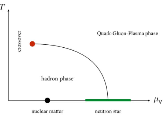
From the order parametersσf and Φ, we can classify phases of the QCD and draw the QCD phase diagram inT-µqplane in which hadron and quark-gluon states are represented. A sketch of the QCD phase diagram is presented in Fig. 1.2; See also Refs. [15, 16, 17, 18] for further details of the QCD phase diagram.
In the figure, there are two representative phases 5). One is the hadron phase that is realized in the lowT and the lowµqregion. In this phase, quarks
3)It was proved in Ref. [12] that vector-type symmetry, such as U(1)V and SU(2)V, is not spontaneously broken in the QCD (Vafa-Witten theorem).
4)In Ref. [14], it was numerically confirmed thatσf is indeed finite.
5)Throughout this thesis, we do not consider color superconductor phase, where quarks form cooper pair in color space. For the review, see Ref. [19] and references therein.
Figure 1.2: The QCD phase diagram in T-µq plane.
and gluons are confined into hadron and the spontaneous chiral symmetry breaking also takes place; σf ̸= 0 and Φ = 0. Another phase is called Quark- Gluon Plasma (QGP) phase, or simply quark phase, that appears at largeT and/or µq. The feature of this phase is that quarks and gluons are free from the confinement (Φ = 0) and behave as free particles. In addition, chiral symmetry is restored in this phase (σf ∼0).
The change from the hadron phase to the QGP phase can be regarded as a phase transition and occurs at some critical T and µq. Then, two- types of boundary exist, one being the chiral transition line and the other the deconfinement transition line. In particular, the latter is also referred to as a hadron-quark phase transition line, firstly predicted by Cabibbo and Parisi in Ref. [20] based on Hagedorn theory [21]. At µq/T = 0, the hadron- quark phase transition is crossover and takes place at Tc ∼ 171 MeV for the 2-flavor system [22], at Tc ∼ 160 MeV for the 2+1-flavor system [23, 24], respectively. On the other hand, the transition may be first-order for moderate µq, predicted by Asakawa and Yazaki [25]. If this scenario is true, there should be a critical end point (CEP) somewhere in the diagram. The search of a CEP is extensively done [15].
Recently, theoretical investigations of the QCD phase diagram have been made, particularly at µq/T = 0, because of progress of lattice QCD simula- tions explained in Sec. 1.3. In addition to the property of the hadron-quark transition, the behavior of the equation of state (EoS) is also mostly de- termined [26]. Along these lines, thermal properties of hadron and quark matters are steadily clarified at µq/T = 0.
As for µq/T =∞, the EoS for cold and dense matter is essential tool of understanding properties of neutron star physics. In the nucleonic regime, robust studies on EoS of the symmetric and asymmetric nuclear matter were made, and various properties were understood, such as a role of many-body nuclear force [27, 28, 29]. In addition to the nuclear matter, possibility of the
1.3. LATTICE QCD 9 hyperonic matter [29, 30] and the quark matter [31] may exist in the inner core of neutron star. This means that not only light-quark chemical potential µl = (µu+µd)/2 but also isospin chemical potential µiso = (µu−µd)/2 and strange-quark chemical potential µs become finite. In particular, due to the observations of two-solar-mass neutron star in Refs. [32, 33], whether the quark matter exists in the inner core of neutron star or not is extensively discussed. To answer this, it is important to know the phase structure and the interaction between quarks in the finite (µl, µiso, µs) region.
In the theoretical approach, lattice QCD simulations are the most pow- erful tool of extracting information on the quark matter, but the simulations are difficult due to the sign problem. One of solutions to this difficulty is to consider the regions where the sign problem does not occur and information on finite (µl, µiso, µs) are included. From the next section, we discuss lattice QCD simulations with finite (µl, µiso, µs).
1.3 Lattice QCD
LQCD simulations are the first-principle calculation of the QCD formulated by Wilson [35]. It enables us to treat non-perturbative nature of the QCD.
This is the strong points of LQCD simulations and we can obtain solid in- formation on thermal properties of quark matter. In the simulations, the integrand of the QCD grand-canonical partition function ZQCD determines whether the simulations can be performed or not. After introducing the expression of ZQCD to be evaluated, we briefly review framework of LQCD simulations.
1.3.1 QCD grand-canonical partition function
By using the imaginary-time formalism [7] and Eq. (1.6), we can define the QCD grand-canonical partition function as
ZQCD=
∫
DADq¯Dq exp [
−
∫ β
0
dτ
∫
d3x(LQCD−q¯µγˆ 4q) ]
, (1.24) where ˆµ = diag(µu, µd, µs) in flavor space and the functional integral DA means
DA=
∏4 µ=1
DAµ. (1.25)
The quark field is included in Eq. (1.24) as a bilinear form, and hence we can perform the gauss integral for a Grassmann variable. The integral yields
ZQCD=
∫
DA detM(ˆµ)e−SG, (1.26)
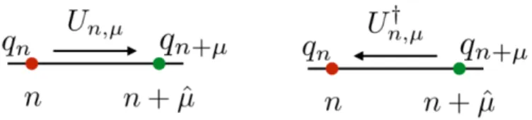
Figure 1.3: Sketch of the link variable. The variable Un,µ goes from lattice point n to n+ ˆµ, while Un,µ† does the inverse direction. The quark field on the point n and n+ ˆµis denoted by qn and qn+µ.
where SG is the pure gauge action andM(ˆµ) is the fermion matrix
M(ˆµ) =M(µu, µd, µs) = γµDµ+ ˆm−µγˆ 4, (1.27) and its determinant is called the fermion determinant.
The QCD thermodynamic potential ΩQCD (per unit volume) is obtained from
ΩQCD=−1
βlogZQCD. (1.28)
Other thermodynamic quantities can be derived from ΩQCD. Also for the expectation value of any physical quantity O, we can take the path-integral representation [7] as
⟨O⟩= 1 ZQCD
∫
DA OdetM(ˆµ)e−SG. (1.29)
1.3.2 Sign problem
In LQCD, the QCD is discretized and formulated on a four-dimensional lat- tice with lattice spacing a. The quark field is putted on each lattice site and the gluon field is expressed by a link variable
Un,µ ≡U(n, n+ ˆµa) = exp [iaAµ(n+ ˆµ/2)], (1.30) where n is the lattice point and ˆµ is the unit vector of µ-direction. The link variable describes the gluon propagating from x tox+ ˆµ. The Hermite conjugate of Eq. (1.30) is written by
Un,µ† =Un+µ,−µ (1.31)
and means the gluon propagating the inverse direction of Un,µ. The gluon field is thus treated so that it connects the neighborhood site; see Fig. 1.3.
By using the link variables, the grand-canonical partition function on the lattice is given by
ZQCD=
∫
DU detM(ˆµ)e−SG, (1.32)
1.4. IMAGINARY CHEMICAL POTENTIAL METHOD 11 i.e., ZQCD is the sum of link variables. In LQCD simulations, the inte- grand P(U) ≡ detM(ˆµ)e−SG is interpreted as a probability function. With this function, the link variable U is generated with the importance-sampling method of Monte-Carlo technique. Hence, we can directly generate the con- figuration of U from the QCD without any approximation.
The probability function P(U) should have positivity in applying the Monte-Carlo technique and it depends on whether the fermion determinant has positivity. For µq = (µu+µd+µs)/3 = 0, the fermion matrix satisfies γ5-hermiticity:
γ5M(0)γ5 = (M(0))†. (1.33) Positivity of the fermion determinant detM(0) is thus ensured and the Monte-Carlo method is available. However, the fermion determinant can be complex when µq ̸= 0, since the relation
(M(ˆµ))†=γ5M(−µˆ∗)γ5, (1.34) or equivalently,
(M(µu, µd, µs))†=γ5M(−µ∗u,−µ∗d,−µ∗s)γ5 (1.35) does not guarantee positivity of the fermion determinant. Hence, it is difficult to access to the finite µq region with LQCD. This is the well-known sign problem [34] and the shortcoming of LQCD.
Some methods of circumventing the sign problem were proposed so far, e.g., the imaginary chemical potential method, the reweighting method, the Taylor expansion method, and so on. Among these methods, we pick up the imaginary chemical potential method.
1.4 Imaginary chemical potential method
In this section, we discuss the imaginary chemical potential method [36, 37].
In particular, we focus on the three regions; (A) imaginary µl region, (B) imaginary µl and µs region, (C) imaginary µl and µiso region. For each region, our main purpose is also presented.
1.4.1 Region (A): 2-flavor case
We first take µu =µd =µl and µs = 0. The imaginary chemical potential is introduced by the replacement µl → iθlT, where θl is a dimensionless light- quark chemical potential. The biggest merit of considering the finiteθlregion is that there is no sign problem. Indeed, Eq. (1.35) ensures the relation
(M(iθlT, iθlT,0))†=γ5M(iθlT, iθlT,0)γ5, (1.36)
Figure 1.4: Sketch of the phase diagram inT-θlplane. The symbolsTpc, TRW mean the deconfinement transition temperature atθl = 0, the RW transition temperature at θl = π/3, respectively. The solid vertical line is the RW transition line and the dotted line stands for the crossover deconfinement transition line.
and the fermion determinant has positivity. Therefore, the integrand ofZQCD
can be interpreted as a probability function, and the usual Monte-Carlo technique works well. Then, we can obtain the θl dependence of physical quantity Ofrom LQCD simulations. The realµldependence of Ois deduced from the analytic continuation, i.e., by replacingθlbyµl/T. This is the basic strategy of the imaginary chemical potential method. When performing the analytic continuation, analyticity of all physical quantities is assumed. It is thus important to know how broad the analytic region is in the finite θl region.
Analyses on the finite θl region were firstly performed by Roberge and Weiss in Ref. [38]. They showed that ZQCD has the periodicity of 2π/3, that is now called Roberge-Weiss (RW) periodicity. It was also proved by Roberge and Weiss that forT < Tpcthe thermodynamic quantity is a smooth function ofθq, while the first-order phase transition takes place atθq = (2k−1)π/3 for T > Tpc, where Tpc is deconfinement-transition temperature at θq = 0. This first-order transition is called the Roberge-Weiss (RW) phase transition. The phase diagram and the quantity deduced from ZQCDthus become periodic in theθqregion and have singularity atθq = (2k−1)π/3; See Fig. 1.4 for a sketch of the phase diagram. The available region to the analytic continuation is thus limited to [0, π/3], due to the RW phase transition for T > Tpc and the RW periodicity forT < Tpc. Then, the imaginary chemical potential method enables us to extract the realµl/T dependence of physical quantity up to the region µl/T ∼1, with small error bars.
To investigate µl ≳ 1, we can consider effective models, but we need to fix a parameter in the models. In virtue of small error bars, LQCD data
1.4. IMAGINARY CHEMICAL POTENTIAL METHOD 13 obtained by using the imaginary chemical potential method have a potential to determine a parameter sharply. In particular, the determination of the strength Gv of the vector-type four-quark interaction
−Gv(¯qγµq)2 (1.37)
is important, since the location of the hadron-quark phase transition line is sensitive to its strength Gv. In Chapter 2, we try to determine the value of Gv from LQCD data on the light-quark number density calculated by the imaginary chemical potential method.
1.4.2 Region (B): 2+1-flavor case
Next, let us consider the imaginary chemical potential method for the 2+1- flavor case. In this case, thes-quark chemical potentialµsis newly introduced as an external parameter, in addition to the light-quark chemical potential.
Even for the 2+1-flavor case, the fermion determinant still possesses positiv- ity for µl =iθlT and µs=iθsT, because
(M(iθlT, iθlT, iθsT))†=γ5M(iθlT, iθlT, iθsT)γ5. (1.38) Hence, the method is useful and applied to the 2+1-flavor case, such as in Refs. [39, 40, 41].
The different point from the 2-flavor case is that the RW periodicity can be lost in the 2+1-flavor case, as shown in Chapter 3. The lack of the periodicity depends on the choice of imaginary θs. In Ref. [39], Bonati et al.
showed that the RW periodicity does not exist when θl ̸= 0 and θs = 0, by calculating the thermodynamic potential in the high-T limit perturbatively.
They also presented a possible phase diagram in T-θl plane, illustrated in Fig. 1.5. In Fig 1.5, it should be noted that the first-order phase transition occurs atθl > π/3, i.e., the transition is delayed whenθs = 0, compared with the 2-flavor case. This indicates that the analytic region can be expanded by breaking the periodicity deliberately and makes the analytic continuation more informative. It is thus interesting to explore when the periodicity is lost, how the actual phase structure is, and how broad the analytic region is.
In Chapter 3, we discuss these questions.
1.4.3 Region (C): 2-flavor case with finite isospin chem- ical potential
We return to the 2-flavor case and consider finite isospin chemical potential µiso. In this case, u- and d-quarks are not degenerate any more and these chemical potentials µu and µd are given by
µu =µl+µiso, µd=µl−µiso. (1.39)
Figure 1.5: The predicted phase diagram in T-θl plane in the 2+1-flavor QCD. Figure is taken from Ref. [39].
For µiso = 0, the relation µl = µu = µd is then recovered, i.e., the system returns to the 2-flavor case. When µiso is finite, the number densities of u- and d-quark are unbalance. This situation can be realized in the inner core of neutron star, where the number density of d-quark is larger than that of u-quark due to the charge neutral condition.
The fermion matrix with finite µiso is obtained as
M(µl, µiso) =γµDµ+ ˆm−µlγ4−µisoγ4τ3, (1.40) where τ3 is the third component of the Pauli matrix. We first set µl = 0 for simplicity and consider real µiso. Equation (1.40) with µl = 0 does not satisfy the usual γ5-hermiticity, but for the case of mu =md =ml, the new relation
(M(0, µiso))† =τaγ5M(0, µiso)γ5τa, a= 1,2 (1.41) guarantees that the fermion determinant detM(0, µiso) has positivity. Here, τa is the first or second components of the Pauli matrix that anticommutes with τ3.
Positivity of the fermion determinant makes LQCD simulations feasible.
Indeed, some works were performed with LQCD simulations at finite real µiso [42, 43]. However, Son and Stephanov demonstrated in Ref. [44] that the charged-pion condensate takes place at µiso =mπ/2 with the pion mass mπ ∼ 138 MeV at vacuum, by using QCD inequalities [45, 46, 47, 48, 12, 49, 50, 51, 52]. Furthermore, it was suggested in Refs. [53, 54] that the charged-pion condensate is related to the severity of the sign problem. LQCD simulations with finite µiso are thus difficult to work when the charged-pion condensate occurs.
1.5. PURPOSE 15 On the contrary, there is no pion condensate at the imaginaryµiso region shown in Ref. [55], applying the chiral perturbation theory. LQCD simula- tions can also be handled in the imaginary µiso region, because of no sign problem there; see Refs. [56, 57]. However, there is no discussion on how the γ5-hermiticity and QCD inequalities are modified, compared with the case of real µiso. In addition, contributions of µl are not included in Refs. [44, 55].
Chapter 4 is devoted to the discussion of the pion condensate not only with real and imaginary µiso but also with imaginary µl.
1.5 Purpose
The purpose of this thesis is summarized as follow:
• In region (A), the strengthGv of the vector-type four-quark interaction is determined from LQCD data on the light-quark number density cal- culated with the imaginary chemical potential method. Furthermore, we study the impact of Gv on neutron-star masses and the hadron- quark phase transition line. These analyses will be done in Chapter 2.
• In region (B), properties of the QCD with imaginary µl and µs are investigated. We first study the condition needed to realize the RW periodicity, inversely, the condition to break the periodicity. After this, we introduce the effective model that possesses the same properties as the QCD. By using the model, we discuss how largely the analytic region can be expanded. These analyses will be performed in Chapter 3.
• In region (C), it is demonstrated that the charged-pion condensate does not occur. In the proof, QCD inequalities are used. In particular, we clarify what determines the presence or absence of the condensate. The proof will be shown in Chapter 4.
Finally, Chapter 5 is devoted to a summary.
line
2.1 Introduction
In this chapter, we analyze the hadron-quark phase transition line in the QCD phase diagram for the 2-flavor case, constructing reliable effective models. As a model of the quark phase, we use the 2-flavor entanglement PNJL (EP- NJL) model [58], which well reproduces LQCD results not only at µl/T = 0 but also at imaginary µl. Therefore, the EPNJL model is a good starting point. Typically, the EPNJL model is composed of the quark part with the scalar-type four-point interaction and the gluon part described by the Polyakov-loop potential. To analyze the hadron-quark phase transition line at high µl, in addition, it is essential to take into account a vector-type four- point interaction with the strength Gv, since the interaction largely affects on properties of the quark matter there. If we include the vector-type inter- action into the model, the strength Gvbecomes an undetermined parameter.
Therefore, we first determine the value of Gv atµl= 0 from LQCD data on the T dependence of the quark number density [59].
The EPNJL model works well to describe not only the quark phase but also the mesonic degree of freedom [60, 61, 62, 63, 64], while cannot treat the baryonic degree of freedom. Therefore, we adopt the two-phase model approach [65, 66] in which the baryonic model is introduced independently.
The two models are connected so as to preserve thermodynamic consistency.
Determination of reliable baryonic model is made from whether the adopted model can reproduce the experimental value of the saturation properties and the observed neutron-star mass with two-solar-mass (2M⊙) [32, 33]. By using the obtained two-phase model, we draw the hadron-quark phase transition line and discuss what can be deduced if we assume that the quark matter exists in the 2M⊙ neutron stars.
16
2.2. EPNJL MODEL WITH VECTOR-TYPE INTERACTION 17
2.2 EPNJL model with vector-type interac- tion
We first formulate the EPNJL model with the vector-type four-quark inter- action. The Lagrangian in Euclidean space-time is defined as
LEPNJL =¯q(γµDµ+ml)q+U(Φ,Φ)¯
−Gs(Φ,Φ)[(¯¯ qq)2+ (¯qiγ5⃗τ q)2] +Gv(Φ,Φ)(¯¯ qγµq)2, (2.1) where q = (u,d)T is the quark field, Dµ = ∂µ +iAµδµ4 is the covariant derivative, and Gs(ϕ,ϕ) and¯ Gv(ϕ,ϕ) are the strength of the scalar- and¯ vector-type interactions with the entanglement vertex [58, 67]:
Gs(Φ,Φ) =¯ Gs
[1−α1Φ ¯Φ−α2(Φ3+ ¯Φ3)]
, (2.2)
Gv(Φ,Φ) =¯ Gv[
1−α1Φ ¯Φ−α2(Φ3 + ¯Φ3)]
. (2.3)
In these expressions, α1 and α2 denote entanglement parameters. In this thesis, we set α1 =α2 = 0.2.
For the Polyakov-loop potentialU(Φ,Φ), we use the logarithmic type [?,¯ 68]:
U(Φ,Φ) =¯ T4 [
−a(T)
2 Φ ¯Φ +b(T) logH(Φ,Φ)¯ ]
, (2.4)
where
a(T) =a0+ (T0
T )
+a2 (T0
T )2
, b(T) = b3 (T0
T )3
(2.5) H(Φ,Φ) = 1¯ −6Φ ¯Φ + 4(Φ3+ ¯Φ3)−3(Φ ¯Φ)2. (2.6) In the potential U(Φ,Φ), the parameter¯ T0 is originally taken to be 270 MeV. This value, however, cannot reproduce LQCD prediction [22, 69] in which the chiral transition temperature Tσ and the deconfinement transition temperature TΦ almost coincide with each other, Tσ ∼ TΦ = Tpc, at µl = 0. We thus rescale T0 from 270 MeV to 190 MeV. Under this rescale, the EPNJL model predicts that the chiral and deconfinement transitions take place simultaneously, which is consistent with LQCD data. In Table 2.1, we tabulate the parameters in the EPNJL model.
We comment on theµl dependence ofT0. In Ref. [70], it is shown by using the quark-meson model and the functional renormalization group method that T0 depends on µl as
T0(µl) = Tτexp [
− 1 α0b(µl)
] , b(µl) = 29
6π − 32µ2l
πTτ2 , α0 = 0.304, Tτ = 1.770(GeV).
(2.7)
a0 a1 a2 b3 T0 [MeV]
3.51 −2.47 15.2 −1.75 190
This represents the backreaction of the quark sector to the gluon sector.
However, the phase structure is not changed qualitatively [71] even if we take into account the dependence. We thus treat T0 as a constant in this thesis.
2.2.1 Thermodynamic potential of EPNJL model
Now, let us perform the mean-field approximation (MFA) to the Lagrangian (??).
We first decompose the bilinear A = ¯qΓq into the expectation value⟨A⟩ and its fluctuation δA around⟨A⟩ as
A=⟨A⟩+δA, (2.8)
where Γ = 1, iγ5⃗τ , γµ. In the MFA, up to the first order of δA is taken into account:
A2 ∼ ⟨A⟩2+ 2δA⟨A⟩
=⟨A⟩2+ 2⟨A⟩(A− ⟨A⟩)
= 2⟨A⟩A− ⟨A⟩2. (2.9)
Furthermore, the rotational invariance in three-dimensional space yields the relation ¯qγµq =δµ4qγ¯ 4q=δµ4q†q, and the parity invariance of vacuum leads to⟨qiγ¯ 5⃗τ q⟩= 0 1). The bilinear included in the Lagrangian (??) thus become (¯qq)2 = 2σqq¯ −σ2, (¯qiγ5⃗τ q)2 = 0, (¯qγµq)2 = 2nlq†q−n2l. (2.10) Here, σ =⟨qq¯ ⟩ is the chiral condensate and nl = ⟨q†q⟩ is the quark number density of the light quark.
By using Eq. (2.10), we can reach the Lagrangian under the MFA:
LMFAEPNJL =¯q(γµDµ+Ml)q+U(Φ,Φ) +¯ Gs(Φ,Φ)σ¯ 2−Gv(Φ,Φ)n¯ 2l, (2.11) where Ml = ml −2Gs(Φ,Φ)σ¯ is the constituent quark mass. Substituting the Lagrangian (2.11) for Eq. (1.24) and using Eq. (1.28), we can obtain the
1)When we consider the isospin chemical potentialµiso, ⟨qiγ¯ 5⃗τ q⟩becomes non-zero for µiso ≥mπ/2 with the pion mass mπ at vacuum. See Refs. [55, 58, 71, 72] for the model analyses under finite µiso.