異なる環境における星形成に関する研究

(1)

九州大学学術情報リポジトリ

Kyushu University Institutional Repository

異なる環境における星形成に関する研究

樋口, 公紀

https://doi.org/10.15017/4059984

出版情報：Kyushu University, 2019, 博士（理学）, 課程博士バージョン：

権利関係：

(2)

Star formation in diﬀerent environments

HIGUCHI Koki

Department of Earth and Planetary Sciences, Graduate School of Science, Kyushu University

February 2020

(3)

Abstract

The environment in which stars are formed varies depending on the location and time of the galaxy. Furthermore, stars are closely related to the formation of galaxies and the chemical evolution of the universe. Therefore, in order to understand the history of the universe, it is necessary to clarify the star formation process. The evolution of collapsing clouds embedded in different environments is investigated using three- dimensional non-ideal magnetohydrodynamics simulations considering different metal- licities (Z/ Z_⊙) and ionization strengths (C_ζ, where C_ζ is a coefficient controlling the ionization intensity). I consider 32 different star-forming environments in combination with Z = 0, 10⁻⁷, 10⁻⁶, 10⁻⁵, 10⁻⁴, 10⁻³, 10⁻², 10⁻¹ Z_⊙ and C_ζ = 0, 0.01, 1, 10, and prepare clouds having different the mass-to-flux ratioµ₀ and the ratio of rotational energy to gravitational energy β₀. I investigate the fragmentation condition in various star-forming environments. I perform 334 runs in total and it is found that 71 models show fragmentation and 15 models show a spiral structure. This study indicates that fragmentation tend to occur with high ionization strength, high metallicity, high µ₀ (µ₀ ≥10, whereµ₀ means the mass-to-flux ratio normalized by the critical value), and high β₀ (β₀ ≥ 3.0×10⁻²). In the collapsing cloud, fragmentation occurs when the following conditions are fulfilled; the high oblateness of core ϵ_ob≥5,µ≥0.6−1.0, and β ≥ 1.0×10⁻². There are some non-fragmentation cases with high µ₀ and β₀. These models are likely to show fragmentation in the later phase. A closed binary system should appear in such models. Furthermore, if these binaries gain a lot of mass and grow into a massive star binary, it can be the origin of the binary black hole.

i

(4)

Chapter 1 INTRODUCTION

1.1 Star-forming environments

There are various star-forming environments in the universe. Within the first billion years after the Big Bang (z ∼9−11), about 40 galaxy candidates have been detected (e.g., Bouwens et al. 2011, Coe et al. 2013, Ellis et al. 2013, Bouwens et al. 2016, Oesch et al. 2016, Lam et al. 2019). These star-forming environments are likely to be the second generation star formation sites. Fig.1.1 shows the promising z >8.5 candidate discovered using Hubble Space Telescope. With the improvement of the accuracy of telescopes, many distant candidate objects have been found. For galaxies with z ≥6, these number is more than 800 (e.g., McLure et al. 2013, Bouwens et al. 2015). These high-redshift galaxies are thought to play an important role in the reionization of the universe (e.g., Stanway et al. 2003, Ishigaki et al. 2015). Starburst galaxies at z ∼ 2 are the most active star formation environment in the universe (e.g., Steidel et al. 1996, 2004, Tacconi et al. 2008) The star-formation rates (SFR) of them exceed 100 solar masses per year, and for example, NAv1.144 galaxy has SFR∼1338M_⊙yr⁻¹, its star- forming activity is very high (Falgarone et al. 2017). In such a diverse environment, various star formation processes are expected. Because the cloud differs depending on the surrounding characteristics, the characteristics of the protostar that is finally formed in should be also different.

(7)

Figure 1.1: Hubble Space Telescope WFC3/IR images of the promising z > 8.5 candidates (Ellis et al. 2013).

1.2 First star v.s. Present-day stars

The ﬁrst star, that is formed from pristine gas at epoch of cosmic dawn (z ∼ 30), is expected to be more massive (M ∼ 10−1000M_⊙; see Fig.1.2) than the present-day star (the typical mass is ≤ 1M_⊙) (Hirano et al. 2014, 2015). The primordial gas has a high temperature due to the lack of coolant (e.g., heavier element and dust). As a result, because of the high gas temperature which is about two orders of magnitude higher than the present-day temperature, the Jeans mass is large. Thus, the typical mass of the ﬁrst star is assumed to be higher than the nearby stars (e.g., Abel et al.

2002, Bromm et al. 2002). The diﬀerence in the stellar mass aﬀects the radiation intensity, thus change the thermal and chemical evolution of the next-generation star- formation site (e.g., Hosokawa et al. 2011, 2012, 2016, Susa et al. 2014). It is important to accurately estimate the mass and multiplicity.

2

(8)

Figure 1.2: Final distribution of the calculated stellar masses for first stars (Hirano et al. 2014). The horizontal axis indicates the mass of stars, and the vertical axis indicates the number. The difference in color represents the difference in protostellar evolution.

1.3 Cloud fragmentation

One important issue is the stellar multiplicity. When fragmentation occurs in a cloud, the stellar mass greatly changes. Dynamical, radiative and chemical feedbacks to the surroundings are roughly limited by the stellar mass (e.g., Baraﬀe et al. 2001, Heger and Woosley 2002, Latif and Khochfar 2019). When a star that is predicted to have a large mass, such as the ﬁrst star, is formed as a binary, the possibility of progenitors of gamma-ray bursts and gravitational wave sources (e.g., Kinugawa et al. 2017) becomes high, which is very important.

Recent numerical simulations of the first star (Pop. III star) have mentioned the possibility of fragmentation. Turk et al. (2009) performed hydrodynamical simulations that start from cosmological initial conditions. They simulated five realization of the first generation of Population III stars (Pop. III.1 stars) and found fragmentation in primordial gas cloud with rotation and turbulence. Pop. III.1 star is formed in pristine clouds unaffected by prior star formation. Clark et al. (2011) explored the effects of turbulence on the Pop. III.1 and Pop. III.2 star formation. Pop. III.2 star is formed

(9)

Figure 1.3: The mass function of Pop. III.1 (left panel) and Pop. III.2 star (right panel) for their simulations (Clark et al. 2011).

in clouds having a high ionization fraction. Pop. III.1 star is easier to fragment than Pop. III.2 star (see Fig.1.3), because there is an adiabatic phase (at n ∼ 10⁷cm⁻³) in Pop. III.2 star formation. Machida et al. (2008a) performed MHD simulations including self-gravity, and indicated that core fragments in the range of β₀ > 10⁶ during the collapse (see Fig.1.4). In addition, Machida et al. (2008b) examined that fragmentation processes in a collapsing primordial cloud using three-dimensional MHD simulations. They showed that fragmentation occurs before protostar formation with Ω_c >10⁻¹⁷(n_c/10³cm⁻³)^2/3s⁻¹ andβ₀ > γ₀. As can be seen, the presence of a magnetic field and rotation greatly changes the picture of star formation (Fig.1.4). In particular, the magnetic field causes magnetic breaking (e.g., Basu and Mouschovias 1994) and outflow (e.g., Tomisaka 2000, Banerjee and Pudritz 2006, Machida et al. 2007, Tomida et al. 2015), and plays an important role for angular momentum transfer in the present- day star formation process.

4

(10)

Figure 1.4: Simulation result for Machida et al. (2008a). Plots of density distribution of each model with models arranged based on the ratio of rotational energy to gravitational energyβ₀ (vertical axis) and the ratio of magnetic energy to gravitational energy γ₀ (horizontal axis).

1.4 Observations in the present-day star-forming region 1.4.1 Magnetic ﬁeld

Magnetic fields play a vital role in the physics of interstellar medium. The magnetic field strength is measured using the Zeeman effect. In our galaxy, the star-forming clouds have smaller µ, which is the mass-to-flux ratio of the initial cloud normalized

(11)

Figure 1.5: The observed mass-to-ﬂux ratios for star-forming clouds (Heiles and Crutcher 2005).

by the critical value,

µ₀ = (M/Φ)

(M/Φ)_cri, (1.1)

where M and Φ are the mass and magnetic flux of the initial cloud, respectively, and (M/Φ)_cri is the ratio of the critical values of these parameters, which is (M/Φ)_cri ≡ (2πG^1/2)⁻¹ (Nakano and Nakamura 1978). Observation shows that µ ≤10 (Crutcher 1999, Heiles and Crutcher 2005, Crutcher et al. 2010: see also Fig.1.5). It is shown that the B_max of the molecular cloud in the vicinity is proportional to the 2/3 power of ncm⁻³ in the range of n > 300 cm⁻³, for example, in molecular cloud cores, B_max is a few 10 µG. On the other hand, since the magnetic field is amplified with the formation of the cosmic structure and the evolution of the star, the higher red-shifted star-forming environment, a field strength becomes weak. Mao et al. (2017) detected coherent µG magnetic fields in the foreground galaxy at z = 0.439. The strength of the magnetic field in the early universe is very weak, less than 1nG, but it is suggested that the magnetic field is locally amplified to about µG as the structure is formed (e.g., Schleicher et al. 2010, Susa et al. 2015). It is comparable to thermal energy and turbulent energy, and magnetic field could be dynamically important.

6

(12)

1.4.2 Multiplicity

Figure 1.6: Carbon abundance for CEMP stars (Arentsen et al. 2019).

The characteristics of stars in our galaxy and others has been investigated through observational studies. Dense molecular cloud cores are initially rotating with rates of β ≤ 0.15 with a mean value of β ∼ 0.02 (Goodman et al. 1993), where β is the parameter defined as the ratio of rotational kinetic energy to gravitational energy, and β ∼ 0.02 indicates that rotation is energetically dominant in the support of the cloud core. In fact, 60 to 80% of the field stars in the galaxy are suggested as binary stars (Duquennoy and Mayor 1991), and it seems that the rotation has an important influence on star formation. On the other hands, when metal-poor stars are observed, these stars are found as carbon-enhanced metal-poor (CEMP) stars. There are two types of CEMP stars, which are CEMP-s and CEMP-no stars, initially defined by Beers and Christlieb (2005). The CEMP-s stars show additional enhancements to the s-process element, while the CEMP-no stars do not show this trend. CEMP-s stars are observed as binary with almost 100% probability (e.g., McClure and Woodsworth 1990, Lucatello et al. 2005). CEMP-no stars are observed as binary with higher absolute carbon abundance with a proportion of 47% and lower absolute carbon content with a probability 18% (Arentsen et al. 2019). Fig.1.6 shows the Carbon abundance for CEMP stars with respect to the Z/ Z_⊙, and there is a tendency that binary is decreasing as

(13)

the metallicity decreases. It is necessary to simulate whether this tendency is real.

8

(14)

Chapter 2 METHODS

2.1 Parameters

I prepare 32 environments characterized by metallicityZ/ Z_⊙and ionization parameter C_ζ. I consider the metallicity in the range of 0 ≤ Z/ Z_⊙ ≤ 10⁻¹ (Z/ Z_⊙ = 0, 10⁻⁷, 10⁻⁶, 10⁻⁵, 10⁻⁴, 10⁻³, 10⁻², 10⁻¹). The ionization strength is deﬁned as

ζ =ζ_CR+ζ_RE,short+ζ_RE,long, (2.1)

ζ_CR=C_ζζ_CR,0exp(−ρR_J/λ), (2.2) ζ_RE,short = 7.6×10⁻¹⁹s⁻¹C_ζ, (2.3) and

ζ_RE,long = 1.4×10⁻²²s⁻¹Z/Z_⊙. (2.4) Eqs.2.2–2.4 show the contribution of cosmic rays, short-lived, and long-lived radioactive elements, respectively. ζCR,0 (= 1×10⁻¹⁷s⁻¹), RJ and λ (= 96 g cm⁻²) mean the cosmic-ray ionization rate in the local interstellar medium, the Jeans length and atten- uation length, respectively (Susa et al. 2015, Higuchi et al. 2018). Cζ is a parameter representing the ionization strength ofζ_CRandζ_RE,short. C_ζ = 1 is deﬁned in the nearby star-forming environment, and Cζ = 0.01 or 10 are adjusted to an ionization intensity corresponding to the ﬁrst galaxy like or starburst galaxy like environment. When Cζ = 0, the contribution of cosmic ray and short-lived radioactive elements disappears

(15)

(in eqs.2.2 and 2.3). In addition, when metallicity becomes zero, the contribution of long-lived radioactive elements also disappears (in eq.2.4), which corresponds to the primitive environment at the beginning of the universe (for details, see Susa et al.

2015). Combining two parameters, which are the metallicity (Z/ Z_⊙ = 0, 10⁻⁷, 10⁻⁶, 10⁻⁵, 10⁻⁴, 10⁻³, 10⁻², 10⁻¹) and the ionization parameter (C_ζ = 0, 0.01, 1, and 10), I investigate 32 collapsing gas clouds embedded in various environments. The model names and physical quantities of each cloud are listed in the Table 2.1–2.4.

2.2 Numerical method and basic equations

As the initial state of star-forming clouds, a critical Bonnor – Ebert (B.E.) density profile (Ebert 1955, Bonnor 1956), which is usually used as the initial condition of cloud (e.g., Matsumoto and Tomisaka 2004, Banerjee and Pudritz 2006), is adopted for each model. This density profile is determined by the central number density n_c and the cloud temperature T_cl. T_cl is determined as the one-zone calculation of the thermal/chemical evolution with different metallicity and ionization strength, and the initial central number density is adopted as n_c,0 = 10⁴cm⁻³. Details are described in Table 2.1–2.4. To promote contraction, the density is set to 1.8 times the critical B.E. density profile (Machida and Hosokawa 2013, Higuchi et al. 2018, 2019). Clouds have initially different radii and masses with different models (for specific value, see Table 2.1–2.4), but the ratio of thermal to gravitational energyα₀, which greatly affects cloud collapse, is the same value (α= 0.47) for all models. In this study, simulation is performed with different ratio of rotational to gravitational energyβ₀ and mass-to-flux ratio µ₀ of the initial cloud in order to investigate the fragmentation process of the 32 collapsing cloud (Tabele 2.1–2.4).

The cloud collapse for each model in Table 2.1–2.4 is calculated using three-dimensional non-ideal MHD nested grid simulations in the same way as Higuchi et al. (2018, 2019).

10

(16)

The following basic equations are implemented in the nested grid code:

∂ρ

∂t +∇ ·(ρv) = 0, (2.5)

ρ∂v

∂t +ρ(v· ∇)v=−∇P − 1

4πB×(∇ ×B)−ρ∇ϕ, (2.6)

∂B

∂t =∇ × [

v×B+ η_AD

|B|²[(∇ ×B)×B]×B−ηOD(∇ ×B) ]

, (2.7)

∇²ϕ= 4πGρ, (2.8)

where ρ, v, P, B, and ϕ denote the density, velocity, pressure, magnetic flux density, and gravitational potential, respectively. The gas pressure P is taken from the table calculated by the one-zone calculation (for details, see Higuchi et al. 2018, 2019). The coefficients of Ohmic resistivity η_OD and ambipolar diffusion η_AD are also obtained from the table. Note that η_OD is referenced from the table as the density argument, while ηAD is referenced as both density and magnetic field strength arguments (Susa et al. 2015, Higuchi et al. 2018). Each grid is composed of (i, j, k) = (64, 64, 32), and mirror symmetry is applied with respect to the z-axis (for a detailed, see Machida et al. 2004, 2005, 2007, 2008a). The finer grid is embedded in the coarser grid and the finer grid is continuously generated so that the Jeans length is resolved at least 16 cells (Truelove et al. 1997). Using this code, the cloud evolution is calculated during collapsing phase (nc ≤ 10¹⁶cm⁻³). I also examine the contribution of the ionization strength, the metallicity, the magnetic field, and rotation of cloud to fragmentation.

(17)

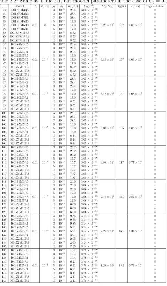
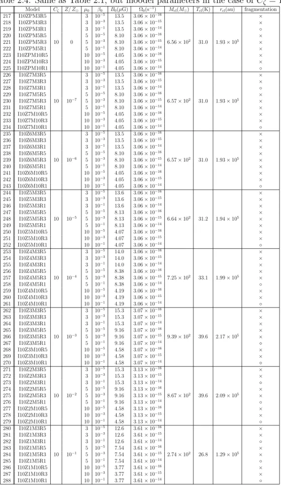
Table 2.1: Model parameters in the case of Cζ = 0. Columns 1 and 2 list the model number and model name, respectively. Columns 3 through 6 list the ionization strength C_ζ, the metallicity Z/ Z_⊙, the ratio of rotational to gravitational energy β₀, and the mass-to-ﬂux ratioµ0, respectively. Columns 7 through 11 list the initial magnetic ﬁeld strengthB₀, the initial angular velocity Ω₀, the cloud massM_cl, the cloud temperature T_cl, and the cloud radius r_cl, respectively. Column 12 lists whether fragment (◦) or spiral (⋄) appear or not (×).

Model Cζ Z/ Z_⊙ µ0 β0 B0(µG) Ω0(s⁻¹) Mcl(M_⊙) Tcl(K) rcl(au) fragmentation

1 I0ZPM3R5 3 10⁻⁵ 34.1 3.05×10⁻¹⁶ ×

2 I0ZPM3R3 3 10⁻³ 34.1 3.05×10⁻¹⁵ ×

3 I0ZPM3R1 3 10⁻¹ 34.1 3.05×10⁻¹⁴ ×

4 I0ZPM5R5 5 10⁻⁵ 20.5 3.05×10⁻¹⁶ ×

5 I0ZPM5R3 0 0 5 10⁻³ 20.5 3.05×10⁻¹⁵ 1.08×10⁴ 198 4.91×10⁵ ×

6 I0ZPM5R1 5 10⁻¹ 20.5 3.05×10⁻¹⁴ ×

7 I0ZPM10R5 10 10⁻⁵ 10.2 3.05×10⁻¹⁶ ×

8 I0ZPM10R3 10 10⁻³ 10.2 3.05×10⁻¹⁵ ×

9 I0ZPM10R1 10 10⁻¹ 10.2 3.05×10⁻¹⁴ ×

10 I0Z7M3R5 3 10⁻⁵ 34.1 3.05×10⁻¹⁶ ×

11 I0Z7M3R3 3 10⁻³ 34.1 3.05×10⁻¹⁵ ×

12 I0Z7M3R1 3 10⁻¹ 34.1 3.05×10⁻¹⁴ ×

13 I0Z7M5R5 5 10⁻⁵ 20.5 3.05×10⁻¹⁶ ×

14 I0Z7M5R3 0 10⁻⁷ 5 10⁻³ 20.5 3.05×10⁻¹⁵ 1.08×10⁴ 198 4.91×10⁵ ×

15 I0Z7M5R1 5 10⁻¹ 20.5 3.05×10⁻¹⁴ ×

16 I0Z7M10R5 10 10⁻⁵ 10.2 3.05×10⁻¹⁶ ×

17 I0Z7M10R3 10 10⁻³ 10.2 3.05×10⁻¹⁵ ×

18 I0Z7M10R1 10 10⁻¹ 10.2 3.05×10⁻¹⁴ ×

19 I0Z6M3R5 3 10⁻⁵ 34.1 3.05×10⁻¹⁶ ×

20 I0Z6M3R3 3 10⁻³ 34.1 3.05×10⁻¹⁵ ×

21 I0Z6M3R1 3 10⁻¹ 34.1 3.05×10⁻¹⁴ ×

22 I0Z6M5R5 5 10⁻⁵ 20.5 3.05×10⁻¹⁶ ×

23 I0Z6M5R3 0 10⁻⁶ 5 10⁻³ 20.5 3.05×10⁻¹⁵ 1.07×10⁴ 198 4.91×10⁵ ×

24 I0Z6M5R1 5 10⁻¹ 20.5 3.05×10⁻¹⁴ ×

25 I0Z6M10R5 10 10⁻⁵ 10.2 3.05×10⁻¹⁶ ×

26 I0Z6M10R3 10 10⁻³ 10.2 3.05×10⁻¹⁵ ×

27 I0Z6M10R1 10 10⁻¹ 10.2 3.05×10⁻¹⁴ ×

28 I0Z5M3R5 3 10⁻⁵ 33.8 3.05×10⁻¹⁶ ×

29 I0Z5M3R3 3 10⁻³ 33.8 3.05×10⁻¹⁵ ×

30 I0Z5M3R1 3 10⁻¹ 33.8 3.05×10⁻¹⁴ ×

31 I0Z5M5R5 5 10⁻⁵ 20.3 3.05×10⁻¹⁶ ×

32 I0Z5M5R3 0 10⁻⁵ 5 10⁻³ 20.3 3.05×10⁻¹⁵ 1.05×10⁴ 194 4.87×10⁵ ×

33 I0Z5M5R1 5 10⁻¹ 20.3 3.05×10⁻¹⁴ ×

34 I0Z5M10R5 10 10⁻⁵ 10.1 3.05×10⁻¹⁶ ×

35 I0Z5M10R3 10 10⁻³ 10.1 3.05×10⁻¹⁵ ×

36 I0Z5M10R1 10 10⁻¹ 10.1 3.05×10⁻¹⁴ ×

37 I0Z4M3R5 3 10⁻⁵ 31.9 3.05×10⁻¹⁶ ×

38 I0Z4M3R3 3 10⁻³ 31.9 3.05×10⁻¹⁵ ×

39 I0Z4M3R1 3 10⁻¹ 31.9 3.05×10⁻¹⁴ ⋄

40 I0Z4M5R5 5 10⁻⁵ 19.1 3.05×10⁻¹⁶ ×

41 I0Z4M5R3 0 10⁻⁴ 5 10⁻³ 19.1 3.05×10⁻¹⁵ 8.75×10³ 172 4.59×10⁵ ×

42 I0Z4M5R1 5 10⁻¹ 19.1 3.05×10⁻¹⁴ ⋄

43 I0Z4M10R5 10 10⁻⁵ 9.56 3.05×10⁻¹⁶ ×

44 I0Z4M10R3 10 10⁻³ 9.56 3.05×10⁻¹⁵ ×

45 I0Z4M10R1 10 10⁻¹ 9.56 3.05×10⁻¹⁴ ◦

46 I0Z3M3R5 3 10⁻⁵ 24.6 3.06×10⁻¹⁶ ×

47 I0Z3M3R3 3 10⁻³ 24.6 3.06×10⁻¹⁵ ×

48 I0Z3M3R1 3 10⁻¹ 24.6 3.06×10⁻¹⁴ ⋄

49 I0Z3M5R5 5 10⁻⁵ 14.7 3.06×10⁻¹⁶ ×

50 I0Z3M5R3 0 10⁻³ 5 10⁻³ 14.7 3.06×10⁻¹⁵ 3.98×10³ 103 3.52×10⁵ ×

51 I0Z3M5R1 5 10⁻¹ 14.7 3.06×10⁻¹⁴ ⋄

52 I0Z3M10R5 10 10⁻⁵ 7.37 3.06×10⁻¹⁶ ×

53 I0Z3M10R3 10 10⁻³ 7.37 3.06×10⁻¹⁵ ×

54 I0Z3M10R1 10 10⁻¹ 7.37 3.06×10⁻¹⁴ ⋄

55 I0Z2M3R5 3 10⁻⁵ 9.83 3.15×10⁻¹⁶ ×

56 I0Z2M3R3 3 10⁻³ 9.83 3.15×10⁻¹⁵ ×

57 I0Z2M3R1 3 10⁻¹ 9.83 3.15×10⁻¹⁴ ⋄

58 I0Z2M5R5 5 10⁻⁵ 5.90 3.15×10⁻¹⁶ ×

59 I0Z2M5R3 0 10⁻² 5 10⁻³ 5.90 3.15×10⁻¹⁵ 2.27×10² 16.4 1.33×10⁵ ×

60 I0Z2M5R1 5 10⁻¹ 5.90 3.15×10⁻¹⁴ ◦

61 I0Z2M10R5 10 10⁻⁵ 2.95 3.15×10⁻¹⁶ ×

62 I0Z2M10R3 10 10⁻³ 2.95 3.15×10⁻¹⁵ ×

63 I0Z2M10R1 10 10⁻¹ 2.95 3.15×10⁻¹⁴ ◦

64 I0Z1M3R5 3 10⁻⁵ 10.3 3.78×10⁻¹⁶ ×

65 I0Z1M3R3 3 10⁻³ 10.3 3.78×10⁻¹⁵ ×

66 I0Z1M3R1 3 10⁻¹ 10.3 3.78×10⁻¹⁴ ×

67 I0Z1M5R5 5 10⁻⁵ 6.20 3.78×10⁻¹⁶ ×

68 I0Z1M5R3 0 10⁻¹ 5 10⁻³ 6.20 3.78×10⁻¹⁵ 1.26×10² 18.1 9.67×10⁴ ×

69 I0Z1M5R1 5 10⁻¹ 6.20 3.78×10⁻¹⁴ ◦

70 I0Z1M10R5 10 10⁻⁵ 3.10 3.78×10⁻¹⁶ ×

71 I0Z1M10R3 10 10⁻³ 3.10 3.78×10⁻¹⁵ ◦

72 I0Z1M10R1 10 10⁻¹ 3.10 3.78×10⁻¹⁴ ◦

12

(18)

Table 2.2: Same as Table 2.1, but moodel parameters in the case of C_ζ = 0.01.

Model Cζ Z/ Z⊙ µ0 β0 B0(µG) Ω0(s⁻¹) Mcl(M⊙) Tcl(K) rcl(au) fragmentation

73 I001ZPM3R5 3 10⁻⁵ 28.4 3.05×10⁻¹⁶ ×

74 I001ZPM3R3 3 10⁻³ 28.4 3.05×10⁻¹⁵ ×

75 I001ZPM3R1 3 10⁻¹ 28.4 3.05×10⁻¹⁴ ×

76 I001ZPM5R5 5 10⁻⁵ 17.0 3.05×10⁻¹⁶ ×

77 I001ZPM5R3 0.01 0 5 10⁻³ 17.0 3.05×10⁻¹⁵ 6.20×10³ 137 4.09×10⁵ ×

78 I001ZPM5R1 5 10⁻¹ 17.0 3.05×10⁻¹⁴ ◦

79 I001ZPM10R5 10 10⁻⁵ 8.52 3.05×10⁻¹⁶ ×

80 I001ZPM10R3 10 10⁻³ 8.52 3.05×10⁻¹⁵ ×

81 I001ZPM10R1 10 10⁻¹ 8.52 3.05×10⁻¹⁴ ◦

82 I001Z7M3R5 3 10⁻⁵ 28.4 3.05×10⁻¹⁶ ×

83 I001Z7M3R3 3 10⁻³ 28.4 3.05×10⁻¹⁵ ×

84 I001Z7M3R1 3 10⁻¹ 28.4 3.05×10⁻¹⁴ ◦

85 I001Z7M5R5 5 10⁻⁵ 17.0 3.05×10⁻¹⁶ ×

86 I001Z7M5R3 0.01 10⁻⁷ 5 10⁻³ 17.0 3.05×10⁻¹⁵ 6.19×10³ 137 4.09×10⁵ ×

87 I001Z7M5R1 5 10⁻¹ 17.0 3.05×10⁻¹⁴ ◦

88 I001Z7M10R5 10 10⁻⁵ 8.52 3.05×10⁻¹⁶ ×

89 I001Z7M10R3 10 10⁻³ 8.52 3.05×10⁻¹⁵ ×

90 I001Z7M10R1 10 10⁻¹ 8.52 3.05×10⁻¹⁴ ◦

91 I001Z6M3R5 3 10⁻⁵ 28.4 3.05×10⁻¹⁶ ×

92 I001Z6M3R3 3 10⁻³ 28.4 3.05×10⁻¹⁵ ×

93 I001Z6M3R1 3 10⁻¹ 28.4 3.05×10⁻¹⁴ ◦

94 I001Z6M5R5 5 10⁻⁵ 17.0 3.05×10⁻¹⁶ ×

95 I001Z6M5R3 0.01 10⁻⁶ 5 10⁻³ 17.0 3.05×10⁻¹⁵ 6.18×10³ 137 4.08×10⁵ ×

96 I001Z6M5R1 5 10⁻¹ 17.0 3.05×10⁻¹⁴ ◦

97 I001Z6M10R5 10 10⁻⁵ 8.51 3.05×10⁻¹⁶ ×

98 I001Z6M10R3 10 10⁻³ 8.51 3.05×10⁻¹⁵ ×

99 I001Z6M10R1 10 10⁻¹ 8.51 3.05×10⁻¹⁴ ◦

100 I001Z5M3R5 3 10⁻⁵ 28.1 3.05×10⁻¹⁶ ×

101 I001Z5M3R3 3 10⁻³ 28.1 3.05×10⁻¹⁵ ×

102 I001Z5M3R1 3 10⁻¹ 28.1 3.05×10⁻¹⁴ ◦

103 I001Z5M5R5 5 10⁻⁵ 16.9 3.05×10⁻¹⁶ ×

104 I001Z5M5R3 0.01 10⁻⁵ 5 10⁻³ 16.9 3.05×10⁻¹⁵ 6.03×10³ 135 4.05×10⁵ ×

105 I001Z5M5R1 5 10⁻¹ 16.9 3.05×10⁻¹⁴ ◦

106 I001Z5M10R5 10 10⁻⁵ 8.44 3.05×10⁻¹⁶ ×

107 I001Z5M10R3 10 10⁻³ 8.44 3.05×10⁻¹⁵ ×

108 I001Z5M10R1 10 10⁻¹ 8.44 3.05×10⁻¹⁴ ◦

109 I001Z4M3R5 3 10⁻⁵ 26.2 3.05×10⁻¹⁶ ×

110 I001Z4M3R3 3 10⁻³ 26.2 3.05×10⁻¹⁵ ×

111 I001Z4M3R1 3 10⁻¹ 26.2 3.05×10⁻¹⁴ ◦

112 I001Z4M5R5 5 10⁻⁵ 15.7 3.05×10⁻¹⁶ ×

113 I001Z4M5R3 0.01 10⁻⁴ 5 10⁻³ 15.7 3.05×10⁻¹⁵ 4.88×10³ 117 3.77×10⁵ ×

114 I001Z4M5R1 5 10⁻¹ 15.7 3.05×10⁻¹⁴ ◦

115 I001Z4M10R5 10 10⁻⁵ 7.87 3.05×10⁻¹⁶ ×

116 I001Z4M10R3 10 10⁻³ 7.87 3.05×10⁻¹⁵ ×

117 I001Z4M10R1 10 10⁻¹ 7.87 3.05×10⁻¹⁴ ◦

118 I001Z3M3R5 3 10⁻⁵ 20.0 3.06×10⁻¹⁶ ×

119 I001Z3M3R3 3 10⁻³ 20.0 3.06×10⁻¹⁵ ×

120 I001Z3M3R1 3 10⁻¹ 20.0 3.06×10⁻¹⁴ ◦

121 I001Z3M5R5 5 10⁻⁵ 12.0 3.06×10⁻¹⁶ ×

122 I001Z3M5R3 0.01 10⁻³ 5 10⁻³ 12.0 3.06×10⁻¹⁵ 2.15×10³ 68.0 2.87×10⁵ ×

123 I001Z3M5R1 5 10⁻¹ 12.0 3.06×10⁻¹⁴ ◦

124 I001Z3M10R5 10 10⁻⁵ 6.00 3.06×10⁻¹⁶ ×

125 I001Z3M10R3 10 10⁻³ 6.00 3.06×10⁻¹⁵ ×

126 I001Z3M10R1 10 10⁻¹ 6.00 3.06×10⁻¹⁴ ⋄

127 I001Z2M3R5 3 10⁻⁵ 9.85 3.14×10⁻¹⁶ ×

128 I001Z2M3R3 3 10⁻³ 9.85 3.14×10⁻¹⁵ ×

129 I001Z2M3R1 3 10⁻¹ 9.85 3.14×10⁻¹⁴ ◦

130 I001Z2M5R5 5 10⁻⁵ 5.91 3.14×10⁻¹⁶ ×

131 I001Z2M5R3 0.01 10⁻² 5 10⁻³ 5.91 3.14×10⁻¹⁵ 2.29×10² 16.5 1.34×10⁵ ×

132 I001Z2M5R1 5 10⁻¹ 5.91 3.14×10⁻¹⁴ ◦

133 I001Z2M10R5 10 10⁻⁵ 2.95 3.14×10⁻¹⁶ ×

134 I001Z2M10R3 10 10⁻³ 2.95 3.14×10⁻¹⁵ ×

135 I001Z2M10R1 10 10⁻¹ 2.95 3.14×10⁻¹⁴ ◦

136 I001Z1M3R5 3 10⁻⁵ 10.4 3.78×10⁻¹⁶ ×

137 I001Z1M3R3 3 10⁻³ 10.4 3.78×10⁻¹⁵ ×

138 I001Z1M3R1 3 10⁻¹ 10.4 3.78×10⁻¹⁴ ◦

139 I001Z1M5R5 5 10⁻⁵ 6.21 3.78×10⁻¹⁶ ×

140 I001Z1M5R3 0.01 10⁻¹ 5 10⁻³ 6.21 3.78×10⁻¹⁵ 1.28×10² 18.2 9.72×10⁴ ×

141 I001Z1M5R1 5 10⁻¹ 6.21 3.78×10⁻¹⁴ ◦

142 I001Z1M10R5 10 10⁻⁵ 3.11 3.78×10⁻¹⁶ ×

143 I001Z1M10R3 10 10⁻³ 3.11 3.78×10⁻¹⁵ ◦

144 I001Z1M10R1 10 10⁻¹ 3.11 3.78×10⁻¹⁴ ◦

異なる環境における星形成に関する研究