ペルー地磁気稠密観測網に基づく赤道ジェット電流モデルの開発

(1)

九州大学学術情報リポジトリ

Kyushu University Institutional Repository

松下, 拓輝

https://doi.org/10.15017/1931715

出版情報：Kyushu University, 2017, 博士（理学）, 課程博士バージョン：

権利関係：

(2)

Development of an Equatorial Electro-Jet model based on the dense Peruvian magnetometer array

A THESIS SUBMITTED

BY

HIROKI MATSUSHITA TO

THE DEPARTMENT OF EARTH AND PLANETARY SCIENCES GRADUATE SCHOOL OF SCIENCE

IN PARTIAL FULFILLMENT OF THE REQUIREMENTS FOR THE DEGREE

OF

DOCTOR OF SCIENCE KYUSHU UNIVERSITY

FUKUOKA, JAPAN MARCH 2018

(3)

Abstract

The equatorial electrojet (EEJ) is an eastward-flowing electric current in the equatorial region of the Earth’s ionosphere. It is well known as the source of the abnormal enhancement of the daily variation during geomagnetic quiet time at the magnetic dip equator.

It was reported that equatorial enhancement has been observed not only in the daily variation of the Earth’s magnetic field but also in geomagnetic-disturbance phenomena such as DP2 and SSC. Therefore, the development of a model to represent such latitudinal profiles is important for space weather studies.

Although past researchers have investigated the latitudinal profile of the EEJ using the magnetic data of a Low Earth Orbit (LEO) satellite, it was difficult to investigate its time development due to the characteristics of an LEO satellite. By contrast, the magnetic data on the ground had important roles in the investigation into the time development of a phenomenon or a magnetic local time (MLT) structure since these data are fixed to a certain coordinate system and are continuously derived there. However, it was difficult to identify whether an increase or decrease in the magnetic field variation was caused by the change of current intensity or the size of the current such as the width.

The MAGnetic Data Acquisition System (MAGDAS), which was organized by the International Center for Space Weather Science and Education (ICSWSE), is the largest network of ground magnetometers in the world. MAGDAS was expanded to Peru and the dense magnetometer array in Peru was developed. As a result, we developed a model that continuously derives the latitudinal profile of the EEJ using that data. The best set of parameters for the EEJ model was determined using the method of least squares between the observed field and the calculated field from the modeled EEJ current. The EEJ model was evaluated using Swarm data, which is one of LEO satellite. The data was taken from the Swarm satellite during the portion of its longitudinal orbit that coincided with the Peruvian longitude. The dense Peruvian magnetometer array has been in operation since 2016, and therefore, the events that were selected were amongst those observed in 2016. In total, 33 events were selected, and the results showed good correspondence between the modeled field and the Swarm-observed field between 9 a.m. and 11 a.m. PET while discrepancies at other local times (LTs) may indicate the possibility that the current differs depending on the altitude, i.e., the current on the ground is different from that at Swarm altitude.

(4)

Using the derived model, the correlation between the estimated current density of the EEJ and the amplitude of the equatorial enhancement of the ground magnetic data was shown.

Furthermore, it was shown that the width of the EEJ and the position of the EEJ axis tend to converge at a certain value when the amplitudes of the equatorial enhancement or the peak current density become larger. This kind of trend has also been reported by previous studies, and it is not inconsistent with our results. This result may indicate that the equatorial enhancement disappears and the Sq variation becomes more dominant when the amplitude of the field is small. It is possible that, for this reason, a correlation between the current density and F10.7, which is a parameter used to evaluate the strength of ionization, was not observed.

This study has a great impact on investigations into the EEJ since details of the EEJ’s structure such as its width or current density are available in quasi-real time. It is expected that this model will have play an important role in space weather studies as a tool to monitor the electromagnetic structure in the ionosphere. Moreover, this study showed that our developed EEJ model reveals the possible existence of another current system at different altitudes through the comparison with the Swarm satellite data.

(5)

Acknowledgement

The author wishes to express his gratitude to his supervisor, Assoc. Prof. Akimasa Yoshikawa for his guidance during the course of this research. I’m deeply grateful for his patient supervision and much encouragement. I am also indebted to Assoc. Prof. Kawano, Assoc. Prof. Watanabe for their helpful comments and encouragement for the study during the seminar. The author is also grateful to Dr. Uozumi, Dr. Abe, and Dr. Fujimoto for their invaluable assistance in my research. Grateful thanks are expressed to all of them.

MAGDAS/CPMN magnetic data were provided by the principle investigator of

MAGDAS/CPMN project (http://magdas.serc.kyushu-u.ac.jp/). I also deeply thank the local corroborators of the MAGDAS project in Peru. Dr. Jose Ishitsuka, a staff of IGP, could support to develop the magnetometer array in Peru. Dr. Marco Milla and Mr. Oscar Veliz from IGP also could help a lot to maintain the instruments. Ingr. Victor Alvarado from UNAS helped us for the installation work in TMA, and could do maintenance of the

instruments. The ground magnetic data at PIU, NAZ, ANC and ARE were provided by IGP.

The Swarm data, which is very important in this study as well, were provided by ESA. The author express his gratitude to them.

Hiroki Matsushita Kyushu University 2018

(6)

List of tables

TABLE 2.1LIST OF THE STATIONS THAT SUPPLIED THE MAGNETIC DATA USED IN THIS STUDY ... 27 TABLE 3.1EVENTS LIST FOR COMPARISON WITH LEO DATA ... 33 TABLE 3.2AVERAGED PARAMETERS OF THE EEJ STRUCTURE DERIVED FROM GROUND MAGNETIC DATA (TOP

VALUE IN EACH CELL), AND LEO MAGNETIC DATA (BOTTOM VALUE IN EACH CELL) AT DIFFERENT LOCAL TIMES ... 43

(8)

List of figures

FIGURE 1.1A SCHEMATIC OF THE GENERATION MECHANISM OF THE EEJ, WHERE E1 AND E2 REPRESENT THE EASTWARD ELECTRIC FIELD AND THE VERTICAL POLARIZATION ELECTRIC FIELD IN THE IONOSPHERE. Σ_H AND Σ_P ARE THE HALL CONDUCTIVITY AND THE PEDERSEN CONDUCTIVITY, WHILE B REPRESENTS THE LINE OF THE FORCE OF MAGNETIC FIELD ... 12 FIGURE 1.2THE SCHEMATIC OF THE TRIANGULAR EEJ MODEL (TAKEN FROM SUZUKI AND MAEDA,1968) ... 19 FIGURE 1.3THE LATITUDINAL PROFILE OF RICHMOND’S EEJ MODEL (INDICATED BY CROSSES IN BOTH OF PANELS)

WITH THE LATITUDINAL PROFILES OF (A) THE FOURTH-DEGREE INTENSITY MODEL, AND (B) THE PARABOLIC INTENSITY MODEL (TAKEN FROM FAMBITAKOYE AND MAYAUD,1976) ... 20 FIGURE 1.4(A)A CONTOUR PLOT OF THE EEJ CURRENT DENSITY (A KM^-2) RELATIVE TO THE PEAK DENSITY (A

KM^-2) FOR Α=-2,Β=0, WHERE EASTWARD (WESTWARD) CURRENT IS DENOTED BY SOLID (BROKEN)

CONTOUR LINES. (B)A LATITUDINAL VARIATION OF THE EEJ CURRENT DENSITY FOR Α=-2. (C)SAME AS (B) BUT FOR Α=0 (TAKEN FROM ONWUMECHILI,1965A,B) ... 22 FIGURE 2.1CALCULATED CURRENT MODELS FOR DIFFERENT PARAMETERS, WHERE PEAK CURRENT DENSITY IS

VARIED ON THE LEFT, THE PARAMETER RELATED TO WIDTH IS VARIED IN THE MIDDLE AND THE PARAMETER RELATED TO THE SHAPE IS VARIED ON THE RIGHT ... 25 FIGURE 2.2CALCULATED MODELS OF THE MAGNETIC FIELDS ON THE GROUND FOR DIFFERENT PARAMETERS

VARIED IN THE SAME MANNER AS IN FIGURE 2.1 ... 25 FIGURE 2.3MAP OF THE STATIONS THAT SUPPLIED THE MAGNETIC DATA FOR THIS STUDY ... 27 FIGURE 3.1ILLUSTRATION OF AN ORBITAL INCLINATION (TAKEN FROM “CATALOG OF EARTH SATELLITE ORBITS”

BY NASA) ... 30 FIGURE 3.2A NORTHWARD MAGNETIC FIELD OBSERVED BY SWARM (BLUE) AND THAT MODELED BY IGRF12

(GREEN) AVERAGED BETWEEN 10 A.M.-2 P.M. LOCAL TIME AND BETWEEN GEOGRAPHIC LONGITUDES OF -70

AND -80, WHERE THE MINUS INDICATES A WESTWARD DIRECTION (TOP),RESIDUAL BETWEEN THE

OBSERVATIONS BY SWARM AND THE IGRF12-MODELED DATA (BOTTOM). ... 31 FIGURE 3.3DAILY VARIATIONS OF THE GROUND MAGNETIC DATA FOR CASE 1(LEFT), AS WELL AS A MAP OF THE

STATIONS AND THE LEO ORBIT (RIGHT) ... 35 FIGURE 3.4LATITUDINAL PROFILES OF THE MODEL VALUES (BLACK SOLID LINE) AND THE OBSERVED VALUES

(RED STAR) OF THE EEJ-ORIENTED MAGNETIC FIELD FOR CASE 1 ... 35 FIGURE 3.5LATITUDINAL PROFILE OF THE MODELED FIELD FOR THE LEO ALTITUDE (BLUE) AND THE OBSERVED

LEO MAGNETIC DATA FOR CASE 1 ... 36 FIGURE 3.6LATITUDINAL PROFILE OF THE ESTIMATED EEJ CURRENT STRUCTURE FROM GROUND MAGNETIC DATA

(BLUE) AND LEO MAGNETIC DATA (GREEN) FOR CASE 1 ... 36 FIGURE 3.7SAME AS IN FIGURE 3.3, BUT FOR CASE 2 ... 38

(9)

FIGURE 3.8SAME AS IN FIGURE 3.4, BUT FOR CASE 2 ... 38 FIGURE 3.9SAME AS IN FIGURE 3.5, BUT FOR CASE 2 ... 39 FIGURE 3.10SAME AS IN FIGURE 3.6, BUT FOR CASE 2 ... 39 FIGURE 3.11COMPARISON BETWEEN MODELED FIELDS OBTAINED FROM GROUND MAGNETIC DATA (BLUE) AND

SWARM MAGNETIC DATA (GREEN) ... 42 FIGURE 3.12COMPARISON BETWEEN THE ESTIMATED CURRENT STRUCTURE FROM GROUND MAGNETIC DATA

(BLUE) AND SWARM MAGNETIC DATA (GREEN) ... 42 FIGURE 3.13LATITUDINAL PROFILES OF THE MODEL FIELD (BLUE SOLID LINE), THE MODEL FIELD INCLUDING AN

INDUCED CURRENT EFFECT (BLUE BROKEN LINE) AND THE OBSERVED FIELD DATA (RED DOTS) ALL FOR THE HORIZONTAL COMPONENT ... 46 FIGURE 3.14LATITUDINAL PROFILES OF THE MODEL FIELD (BLUE SOLID LINE), THE MODEL FIELD INCLUDING AN

INDUCED CURRENT EFFECT (BLUE BROKEN LINE) AND THE OBSERVED FIELD DATA (RED DOTS) FOR THE VERTICAL COMPONENT ... 46 FIGURE 3.15THE OBSERVED EEJ FIELD FROM THE SWARM SATELLITE AND THE FIELD WHICH INCLUDES THE

INDUCED CURRENT EFFECT ... 47 FIGURE 3.16LATITUDINAL VARIATION OF THE EEJ FIELD OBSERVED BY THE SWARM SATELLITE (GREEN SOLID

LINE), THE MODEL FIELD UNDER THE ASSUMPTION OF 110 KM ALTITUDE OF THE EEJ(BLUE SOLID LINE) AND THE MODEL FIELD FOR A 195 KM ALTITUDE OF THE EEJ(BLUE BROKEN LINE) ... 47 FIGURE 3.17THE HEIGHT PROFILE OF THE IONOSPHERIC CONDUCTIVITIES, WHERE THE BLUE-, GREEN-, RED- AND

BLACK-COLORED PLOTS CORRESPOND TO PEDERSEN CONDUCTIVITY,HALL CONDUCTIVITY,COWLING CONDUCTIVITY AND PARALLEL CONDUCTIVITY, RESPECTIVELY, AT 12 P.M. LOCAL TIME ON FEBRUARY 12, 2016. THE LOCATION IS GIVEN BY (-12.0,-75.0) DEGREES OF GEOGRAPHIC LATITUDE AND LONGITUDE .. 48 FIGURE 4.1LONG-TERM VARIATIONS OF THE EEJ STRUCTURAL PARAMETERS.IN ORDER FROM THE TOP TO

BOTTOM: THE OBSERVED EQUATORIAL ENHANCEMENT OF THE FIELD AT HUA, THE PEAK AMPLITUDE OF THE

EEJ CURRENT, THE WIDTH OF THE EEJ AND THE POSITION OF THE EEJ AXIS ... 51 FIGURE 4.2THE SCATTER PLOT OF THE EQUATORIAL ENHANCEMENT VERSUS THE PEAK AMPLITUDE OF THE EEJ

CURRENT ... 51 FIGURE 4.3THE SCATTER PLOT OF THE EQUATORIAL ENHANCEMENT VERSUS THE WIDTH OF THE EEJ CURRENT 52 FIGURE 4.4THE SCATTER PLOT OF THE EQUATORIAL ENHANCEMENT VERSUS THE POSITION OF THE EEJ AXIS .... 52 FIGURE 4.5SCATTER PLOT OF F10.7 VERSUS THE EQUATORIAL ENHANCEMENT (TOP LEFT), THE PEAK AMPLITUDE

OF THE EEJ CURRENT (TOP RIGHT), THE WIDTH OF THE EEJ(BOTTOM LEFT) AND THE POSITION OF THE EEJ

AXIS (BOTTOM RIGHT) ... 53 FIGURE 5.1DAILY VARIATION OF THE HORIZONTAL COMPONENT OF THE MAGNETIC FIELD ON JULY 21,2016

DURING A GEOMAGNETICALLY QUIET TIME (TOP LEFT).SAME AS IN (TOP LEFT) BUT FOR THE VERTICAL COMPONENT (TOP RIGHT) AND THE EQUATORIAL ENHANCEMENT OF THE DAILY VARIATION DERIVED BY

(10)

SUBTRACTING THE VARIATION AT PIU, WHICH IS USED AS THE REFERENCE STATION OF SQ VARIATION

(BOTTOM) ... 56 FIGURE 5.2AN EEJ CURRENT DENSITY DISTRIBUTION IN LOCAL TIME-GG LATITUDE FLAME ON JULY 21,2016 . 57 FIGURE 5.3SAME AS IN FIGURE 5.1 EXCEPT THAT THE DATA IS FOR OCTOBER 11,2016 WHEN THE CEJ WAS

OBSERVED IN MORNING ... 59 FIGURE 5.4SAME AS IN FIGURE 5.2 BUT FOR THE DATA FROM OCTOBER 11,2016 ... 60 FIGURE 5.5TIME SERIES OF THE DST INDEX BETWEEN OCTOBER 12 AND OCTOBER 17 IN 2016, WHERE T₀, T₁, T₂,

AND T₃ ARE DEFINED BY THE DATE IN PERU. ... 63 FIGURE 5.6SAME AS THOSE IN FIGURE 5.1 EXCEPT THAT THE DATA ARE FOR OCTOBER 12,2016 BEFORE THE MAIN PHASE OF THE GEOMAGNETIC STORM ... 63 FIGURE 5.7SAME AS IN FIGURE 5.2 BUT FOR THE DATA FROM OCTOBER 12,2016 ... 64 FIGURE 5.8SAME AS THOSE IN FIGURE 5.1 EXCEPT THAT THE DATA ARE FROM OCTOBER 13,2016 DURING THE

MAIN PHASE OF THE GEOMAGNETIC STORM ... 65 FIGURE 5.9SAME AS IN FIGURE 5.2 BUT FOR THE DATA FROM OCTOBER 13,2016 ... 66 FIGURE 5.10SAME AS THOSE IN FIGURE 5.1 EXCEPTING THAT THE DATA ARE FROM OCTOBER 14,2016 DURING

THE RECOVERY PHASE OF THE GEOMAGNETIC STORM ... 67

(11)

1. Introduction

1.1 Classical theory of the equatorial electrojet (EEJ)

A noticeably enhanced horizontal magnetic field near the dip equator during daytime has been detected by magnetometers on the ground (e.g. Bartles and Johnston. 1940a,b). This enhancement of the field is caused by an intense eastward electric current, which flows in the E region of the ionosphere along the dip equator, known as the equatorial electrojet (EEJ).

There are generally two reasons for the highly intense EEJ: the geometry of the Earth’s magnetic field lines and higher effective conductivity. The generation mechanism of the EEJ is illustrated in figure 1.1, and is explained as follows. Solar extreme ultraviolet (EUV) radiation and the ionization of the atmosphere are active in the daytime and are most active around the equator. Tidal winds in the E region of the ionosphere produce an electric field according to

𝐸 = 𝑈×𝐵 (1−1)

where 𝑈 is the velocity of the winds and 𝐵 is the magnetic field. As an ion (electron) is carried by this electric field and is charged at dawn (dusk) side, the eastward electric field from dawn to dusk can be set up along the dip equator. This eastward electric field then causes a Pedersen current to flow parallel to the electric field and a Hall current to flow downwards or perpendicular to both the electric field and the magnetic field. The Pedersen and Hall currents are denoted by 𝜎_!𝐸_! and 𝜎_!𝐸_! in figure 1.1, respectively. The downward Hall current cannot cross the boundaries, which are in the form of non-conducting atmosphere at the bottom of the slab and effectively collisionless plasma at the top of the slab in the figure. This interruption of electric current causes the accumulation of negative charge at the top of the slab and positive charge at the bottom of the slab, that is, an upward electric field denoted by 𝐸_! in figure 1.1. Subsequently, a Pedersen current and a Hall current, which are denoted by 𝜎_!𝐸_! and 𝜎_!𝐸_! in figure 1.1, flow upward and eastward, respectively. The latter Pedersen current will cancel the former Hall current in a steady state, while the latter Hall current will enhance the former Pedersen current. The total vertical current and zonal current are given by equation (1−2) and equation (1−4), respectively:

𝐽_!= 𝜎_!𝐸_! −𝜎_!𝐸_! =0 (1−2)

(12)

𝐸_! = 𝜎_!

𝜎_!𝐸_! (1−3)

𝐽_! =𝜎_!𝐸_!+𝜎_!𝐸_! =𝜎_!𝐸_! (1−4)

where 𝜎_! is the Cowling conductivity (Hirono, 1950a,b; Hirono, 1952; Hirono, 1953), which is defined as 𝜎_! ≡^!^!^!_!^!!^!^!

!! . Since the generation of the vertical electric field proceeds most efficiently at the dip equator, where the magnetic field lines are perpendicular to the boundaries, and Cowling conductivity is at a maximum around the equator owing to the ionization by EUV radiation, the observed enhancement is also at a maximum at the equator.

The resulting strong eastward electric current is called the EEJ, which is generally described to flow in the narrow region between -3 and 3 degrees of dip latitude, and produces a noticeably enhanced ground magnetic field.

(13)

Figure 1.1 A schematic of the generation mechanism of the EEJ, where E1 and E2 represent the eastward electric field and the vertical polarization electric field in the ionosphere. σ_H and σ_P are the Hall conductivity and the Pedersen conductivity, while B represents the line of the force of magnetic field

(14)

1.2 Reviews of EEJ studies

Although the basic generation mechanism of the EEJ can be explained as in section 1.1, there are still interesting features of the EEJ, such as local time (LT) variation/long-term variation/day-to-day variability of the amplitude, the longitudinal dependency of the EEJ, and the structure of EEJ that require investigation. Accordingly, the past studies related to these features are introduced in the following subsections for each different method or tool.

1.2.1 Ground magnetic data

As mentioned above, the equatorial enhancement was originally noticed in ground magnetic data. Later, Chapman (1951) reported that the large range of the horizontal component of the daily variation in the magnetic field at Huancayo indicates the existence of an intense eastward current above it, which he named the EEJ. Since the advantage of ground magnetic data for EEJ studies is temporal variation, the relationship between the range of the horizontal component and the solar activity or its seasonal dependency has been investigated in various papers. Yamazaki et al., (2010), using 10 years of datasets, revealed good correlation between F10.7, which is well known as the proxy of solar EUV radiation, and the EEJ variation at Davao in the Philippines whose dip latitude is -0.84 degrees. They found the correlation coefficient to be 0.53. They also found predominant semiannual variation of the EEJ, that is, the peak amplitude could be seen in spring and in fall. This feature was also reported by Stening (1995a), and it is explained as the effect of both semiannual changes in ionospheric conductivity (Wagner et al., 1980) and diurnal tidal wind fields in the middle atmosphere (Burrage et al., 1995). Moreover, Fujimoto et al., (2016) also investigated the relationship between F10.7 and the EEJ variation at Ancon in Peru including a geomagnetically disturbed day using the EE index which was introduced by Uozumi et al., (2008) as an index to monitor EEJ activity. They found that they had similar trends. It should be noted that Yamazaki et al., (2010) and Fujimoto et al., (2016) used the daily range of the northward component as the EEJ variation without separating the global-Sq field and the local-EEJ field. Meanwhile, Hamid et al., (2013) found that the correlation coefficient between F10.7 and the EEJ variation in the Philippines was 0.43, which was calculated using the two-station method wherein the field outside of the dip equator was subtracted from the field at the dip equator.

1.2.2 Low Earth Orbit (LEO) satellite magnetic data

It is difficult to use LEO magnetic data to investigate the temporal variation of the EEJ at a particular location since the LEO satellites orbit different longitudes with every rotation.

(15)

They do, however,they moves through very fast in every orbit very quickly. Therefore, it can be said that the LEO data observe a kind of snap shot of the latitudinal profiles, that is, spatial variation. In addition to the spatial variation, the aspects of the EEJ structure, such as the current density or intensity and the width of the EEJ also can also be estimated using by LEO data. The EEJ variation in the LEO data was observed as a negative depression of the magnetic field of northward component since satellites orbit above eastward flowing EEJ, and the observations by Polar Orbiting Geophysical Observatory (POGO) satellites had revealed such characteristics (Cain and Sweeney, 1973; Onwumechili and Agu, 1980, 1981a,b). Jadhav et al., (2002) studied the EEJ current structure in detail using the Ørsted satellite data, and they found an average height-integrated current density of around 0.20 A/m and very large dispersion of the width of the EEJ. On the other hand, Luhr et al., (2004) found that the current density was 0.15 A/m using the measurements from the CHAllenging Minisatellite Payload (CHAMP) satellite, which is smaller than the value found by Jadhav et al., (2002). They concluded that this discrepancy was due to different current models being adopted As they adopted a series of line current as the EEJ while Jadhav et al., (2002) adopted a continuous distribution of current as the EEJ. The width of the EEJ estimated by Luhr et al., (2004) showed smaller deviation than previous results (Jadhav et al., 2002;

Onwumechili, 1967). They mentioned that previous studies included a geometric effect since the EEJ is tilted in a certain area. As for the relationship between the width and the peak current density, Luhr et al., (2004) revealed that the width of the EEJ becomes larger with higher amplitudes of the peak current density while Onwumechili and Agu, (1981b) reported an inverse trend. Luhr et al., (2004) also found that the close linear relationship between the current density and the current intensity was not constant. Therefore, they concluded that larger currents could flow at longitudes with larger Cowling-channel cross sections.

1.2.3 In-situ sounding rocket-borne observation data

Rocket measurements allow the height profile of the EEJ to be studied while it is difficult to obtain the temporal and spatial variations. Maynard and Cahill, (1965) performed rocket experiments over the dip equator in India, and they found the peak current density at 105 km and 109 km during the ascent and descent, respectively. The lower edge and upper edge of EEJ current density were also detected in their study at 89 km and 136 km from the ground, respectively. Shuman, (1970) also performed a rocket experiment near the dip equator in Peru, and found that the peak amplitude of the current density was observed at 106 km.

Onwumechili, (1992d) revealed a linear relationship between the width of the EEJ and the

(16)

peak current density, that is, the larger (smaller) the amplitude of the peak current density, the thicker (thinner) the EEJ will be.

1.3 Temporal variation of the EEJ

As mentioned above, the use of ground-based magnetic data has an advantage for studying the temporal variation of the EEJ. Hereafter, this temporal variation is briefly introduced. LT variations of the normal EEJ and time developments of the EEJ during a storm/substorm are used to represent the temporal variation of the EEJ during a quiet time and a disturbed time, respectively.

1.3.1 LT variation during a quiet time

The observation of the EEJ variation on the ground, which is an abnormal enhancement of the amplitude of the daily magnetic variation, started in 1922 at Huancayo, Peru by the Department of Terrestrial Magnetism of the Carnegie Institution of Washington. Chapman (1951) explained the feature of LT variation of the EEJ as follows; “the Sq(H) variations during the night are small, and during the day they consist of a rise to and a fall from maximum value at about 11 a.m.” Although the “Sq(H)” in Chapman (1951) included both the local-EEJ field and the global-Sq field, Manoj et al. (2006) also revealed in their paper that the local-EEJ field derived from the difference between values obtained from magnetometer observatories located near the dip equator and off the dip equator showed a similar variation, which is the peak at 11 a.m.

1.3.2 Time developments of the EEJ during a disturbed time

The response of low-latitude electrodynamics to high-latitude geomagnetic activity such as a substorm has been studied using plasma drift measurements at Jicamarca (Fejer and Scherliess (1995); Scherliess and Fejer (1997)) as well as ground-based measurements (Kelley et al., (1979); Gonzales et al., (1979); Wei et al., (2012)). Yamazaki and Kosch (2015) examined the response of the EEJ to geomagnetic storms and substorms using long-time series of ground magnetic data since such a response in daytime had not been well studied, statistically. In the paper, they sorted the substorm effects according to the time history of the AE index, which is an index to represent the relative amplitude of substorm provided by World Data Center (WDC) for Geomagnetism, Kyoto, and found that the EEJ was enhanced when the AE index decreased suddenly, which indicated the penetration of a

(17)

high-latitude convection electric field (c.f. Nishida, 1968). They also suggested that the westward EEJ followed by the disappearance of the enhanced EEJ in an hour indicated the existence of disturbance dynamo (c.f. Blanc and Richmond, 1980). Similarly, they also concluded that the westward disturbances of the EEJ during the recovery phase could also be explained by disturbance dynamo. However, the position of the westward disturbance of the EEJ was not revealed since they used data from only one station for the dip equator at a particular longitude.

1.4 The models of the EEJ current and its magnetic field

Originally, Chapman (1951) proposed three types of electric-current models for the EEJ current. These were the line current model, the current ribbon of constant intensity model, and the current ribbon of parabolic intensity model. Subsequently, the current ribbon of triangular intensity model and the current ribbon of fourth-degree intensity model were introduced by Suzuki and Maeda (1968) and Fambitakoye and Mayaud (1976a), respectively.

Onwumechili (1965a,b) then introduced the continuous distribution of current density model.

These models and their magnetic fields are briefly introduced in this section.

1.4.1 Models proposed by Chapman (1951)

At first, an infinitely long straight current was assumed for the EEJ in his study. The lines of force produced by a current of this type are circles around the axis, and are described as follows

𝐵= 0.2𝐼

𝑟 (1−5)

where 𝐼 is total intensity of the current, and 𝑟 is the distance from the axis. Accordingly, the horizontal component 𝐻 and the vertical component 𝑍 are given by

𝐻 = 0.2𝐼𝑧

𝑥^!+𝑧^! (1−6) 𝑍 = 0.2𝐼𝑥

𝑥^! +𝑧^! (1−7)

(18)

where z is the height of the current while x is the distance from the axis to the north.

Chapman (1951) then suggested “a band of uniform current flow” as a more realistic model of the EEJ. In other words, he suggested the current ribbon of constant intensity model in which the current has a width of 2w in the north-south direction and flows eastward. The horizontal component 𝐻 and the vertical component 𝑍 produced by this current are derived from

𝐻 = 0.2𝐽tan^!! 2𝑤𝑧

𝑥^!+𝑧^!−𝑤^! 1−8 𝑍 =0.1𝐽ln𝑧^!+ 𝑥−𝑤 ^!

𝑧^!+ 𝑥+𝑤 ^! 1−9 where 𝐽 is the sheet current density with the units of A km^-2 and x and z are the distances from the axis to the north and upward, respectively. Finally, he suggested “a distributed band of unidirectional current” as the most realistic model of the EEJ. In this model, using the width of current or the latitudinal extent of the current defined by 2𝑤, and 𝐽_! which is the peak current density at x=0, the model current density 𝐽 at the point y is given by

𝐽= 𝐽_! 1− 𝑦^!

𝑤^! −𝑤 ≤𝑥 ≤𝑤 (1−10𝑎)

𝐽=0 𝑥≥𝑤,𝑥≤−𝑤 (1−10𝑏)

Therefore, the magnetic field change of the horizontal component and the vertical component produced by this current at the point (x, z) are given, respectively, by

𝐻= 2𝐽_!𝑧 1−𝑦^! 𝑤^! 𝑧^!+ 𝑥−𝑦 ^!

!

!!

𝑑𝑦 (1−11𝑎)

𝑍=2𝐽_! 1−𝑦^! 𝑤^! 𝑧−𝑦 𝑧^!+ 𝑥−𝑦 ^!

!

!!

𝑑𝑦 (1−12𝑎)

If

tan𝜃_! =𝑧−𝑤

ℎ , tan𝜃_! =𝑧+𝑤 ℎ , Equations (1 – 11a) and (1 – 12a) can be transformed as follows

(19)

𝐻 = 3𝐶

2𝑤^! 𝑤^!−𝑥^!+𝑧^! 𝑥_! −𝑥_! +2𝑥𝑧lnsec𝜃_!

sec𝜃_! −𝑧^! tan𝜃_!−tan𝜃_! (1−11𝑏)

𝑍= 3𝐶

2𝑤^! 𝑤^!−𝑥^!+𝑧^! lnsec𝜃_!

sec𝜃_!−2𝑥𝑧 𝜃_!−𝜃_! +2𝑥𝑧 tan𝜃_!−tan𝜃_!

−1

2𝑧^! tan^!𝑥_!−tan^!𝑥_! (1−12𝑏)

where 𝐶 =4𝑤𝐽_! 3.

1.4.2 The current ribbon of triangular/fourth-degree intensity models

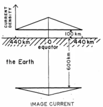
Suzuki and Maeda (1968) proposed the triangular-shaped current, which is shown in figure 1.2, as a simple model of the EEJ, and discussed its reliability by comparing it with theory and rocket measurements. They suggested in the paper that the results of the rocket measurements by Davis et al. (1967) and the theoretical model of the EEJ by Untiedt (1967) could be approximated to a triangular structure of the EEJ from north southward. They also noted, however, that the triangular model could not represent a return current of the EEJ, which had been mentioned in previous papers (e.g. Chapman, 1951; Onwumechili, 1967;

Maynard, 1967). Therefore, they concluded that their model could be regarded as a simplified version of the one by Onwumechili (1967). Fambitakoye and Mayaud (1976) proposed the “fourth-degree distribution current model” for the EEJ. In this model, the current density at 𝑥, which is the distance from the axis to the north, is given by

𝐽 𝑥 = 𝐽_! 1− 𝑥−𝑥_! ^! 𝑎^!

!

(1−13)

where 𝑥_! is the position of the axis, and 𝑎 is the half-width of the current. They confirmed the reliability of the model by comparing the model with the numerical model of the EEJ presented by Richmond (1972), and obtained a very similar latitudinal structure as shown in figure 1.3, which is taken from Fambitakoye and Mayaud (1976). Moreover, they indicated that smaller residuals between Richmond’s model and the fourth-degree current model could be seen than those between Richmond’s model and the parabolic model.

(20)

Figure 1.2 The schematic of the triangular EEJ model (taken from Suzuki and Maeda, 1968)

(21)

Figure 1.3 The latitudinal profile of Richmond’s EEJ model (indicated by crosses in both of panels) with the latitudinal profiles of (a) the fourth-degree intensity model, and (b) the parabolic intensity model (taken from Fambitakoye and Mayaud, 1976)

(22)

1.4.3 The continuous distribution of current density model

Although Chapman (1951) originally suggested three types of models for the EEJ current, Onwumechili (1965a,b) stated that none of Chapman’s models described the equatorial enhancement observed on the ground well and subsequently introduced the “two-dimensional continuous distribution of current density model” as a new model for the EEJ. There are two advantages of this model; the one is the ability to represent the return current of the EEJ.

The other is that it is two-dimensional, that is, it describes the x-z plane, which means that this model is also useful to explain rocket measurements. The current density 𝑗 (A km^-3 for this model at the point (x, z) is given by

𝑗 =𝑗_!𝑎^! 𝑎^!+𝛼𝑥^! 𝑎^!+𝑥^! ^!

𝑏^! 𝑏^!+𝛽𝑧^!

𝑏^! +𝑧^! ^! 𝑦 (1−14)

where 𝑗_! is the peak current density at 𝑥=0,𝑧=0; 𝑎 and 𝑏 are the constant scale lengths along 𝑥 and 𝑧, respectively; and 𝛼 and 𝛽 are dimensionless constants which control the shape of the current along 𝑥 and 𝑧, respectively. Figure 1.4 shows some examples of the latitudinal distribution of this current density from Onwumechili (1965a,b).

1.5 Purpose of this paper

As described previously, there are few studies investigating the latitudinal profile of the EEJ temporally. Hence, the characteristics of the daily magnetic field that change around the dip equator, such as which structural change of the EEJ current contributes to the long-term variation or LT variation are not clear. Accordingly, the dense Peruvian ground-magnetometer array was developed in order to monitor the latitudinal profile of the EEJ continuously. The methodology, containing the model construction and procedure for extracting the EEJ-related magnetic data on the ground, is described in Chapter 2. Chapter 3 details the results of the evaluation of the model using LEO data. The results of the long-term variation of the EEJ structure in 2016 are presented in Chapter 4. Chapter 5 details the LT variations of the EEJ structure during a normal EEJ, a counter EEJ, and a magnetic storm. Finally, the summary and conclusions are presented in Chapter 6 along with the future prospects for research using this EEJ model.

(23)

Figure 1.4 (a) A contour plot of the EEJ current density (A km^-2) relative to the peak density (A km^-2) for 𝜶=−𝟐,𝜷=𝟎, where eastward (westward) current is denoted by solid (broken) contour lines. (b) A latitudinal variation of the EEJ current density for 𝜶=−𝟐. (c) Same as (b) but for 𝜶=𝟎 (taken from Onwumechili, 1965a,b)

(24)

2. Methodology

The EEJ structure, which relates to the width, shape, and total intensity of the EEJ, was estimated by solving the inverse problem of relating the physical models of the magnetic field to the observed magnetic data from the dense magnetometer array near the dip equator in Peru. Each model was produced by changing various parameter values, and the method of least squares was applied to determine which model best described the data. Sections 2.1 and 2.2 explain the details of the models and data from the ground magnetometer array used in this study, respectively.

2.1 The model for the EEJ

In order to estimate the EEJ structure, the continuous thin current shell model (Onwumechili, 1992) was used as the EEJ model and is given by equation (2−1)

𝑗= 𝐽𝑎^! 𝑎^!+𝛼𝑥^!

𝑎^!+𝑥^! ^! (2−1)

where 𝛼,𝑎,𝐽, and 𝑥 express the shape of the current along the meridional line, the latitudinal width of the current, the height-integrated current density at the current axis and the northward distance from the position of the current axis, respectively. The northward and vertical magnetic fields produced by this current are given by equation (2−2) and (2−3), respectively, by solving the equation (2−1) according to Biot-Savart’s law:

− 𝑧𝑋= 1

2𝐾𝑎 𝑣+𝛼𝑣+2𝛼𝑎 𝑢+𝑏 ^!+ 𝑣+𝛼𝑣+2𝑎 𝑣+𝑎 ^!

𝑢+𝑏 ^!+ 𝑣+𝑎 ^! ^! (2−2)

− 𝑥 𝑍=1

2𝐾𝑎 𝑢+𝑏 1+𝛼 𝑢+𝑏 ^!+ 𝑣+𝛼𝑣+3𝑎−𝛼𝑎 𝑣+𝑎

𝑢+𝑏 ^!+ 𝑣+𝑎 ^! ^! (2−3)

where 𝐾 is the constant value, which is described by 𝐾=0.2𝜋𝐽; 𝑢(𝑣) is the absolute value of x(z), which is the northward (vertical) distance from the current axis. The variable 𝑏 is the vertical scale of the current, which is assigned to be zero in this study, and 𝛼,𝑎,𝐽 are defined in the same way as equation (2−1). The model magnetic fields in equation (2−2) were calculated by substituting values from -10 to 0 in steps of 0.1 for 𝛼; values

(25)

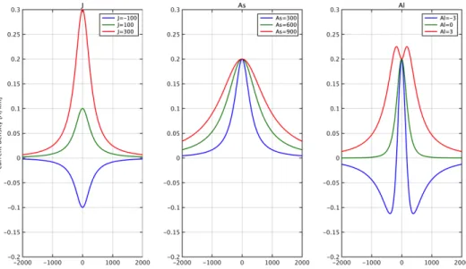
from 200 to 1000 in steps of 10 for 𝑎; and values from 0 to 400 in steps of 1 for 𝐽. The set of values that best explained the EEJ structure obtained from the ground magnetic data using the method of least squares was determined. Figure 2.1 and figure 2.2 display examples of the model-calculated current and magnetic fields for different values of the parameters 𝐽,𝑎,𝛼 from left to right. It should be noted that for each parameter that varies, the other parameters remain at constant values. As figure 2.1 and figure 2.2 indicate, higher values of a and J contribute indicate a wider and higher-density current or amplitude of the magnetic field, and vice-versa. On the other hand, a trend for the contribution of 𝛼 to the current structure is not specifically observed but negative values shape the return current of EEJ.

(26)

Figure 2.1 Calculated current models for different parameters, where peak current density is varied on the left, the parameter related to width is varied in the middle and the parameter related to the shape is varied on the right

Figure 2.2 Calculated models of the magnetic fields on the ground for different parameters varied in the same manner as in figure 2.1

(27)

2.2 Ground magnetic data

The magnetic data on the ground used in this study were provided by the MAGnetic Data Acquisition System/Circum-pan Pacific Magnetometer Network (MAGDAS/CPMN) Group and the Institute del Geo Physico (IGP). Both datasets are available at 1-second and 1-minute time resolution, but 1-hour averaged data of the 1-minute data were used in this study. As shown in Figure 2.3, seven stations located near the dip equator were mainly used, and the location of every stations and of the dip equator is shown by blue-colored circle and a red-solid line, respectively. The red broken lines in the figure show the positions of the edges of the EEJ as mentioned by previous researchers ( Onwumechili, 1992). The information for every station is also summarized in Table 2.1. As the original data of the magnetic field include various effects such as the Sq current, the main field of the Earth, and the

magnetospheric current, the effect of the EEJ had to be extracted. In order to remove these extraneous effects, the magnetic data at Piura, the mean values of the magnetic data from each station for the nighttime between 6 p.m. and 6 a.m., LT in a day and the Dst index, which was introduced by Sugiura & Kamei, (1981) as an index for monitoring the global disturbed magnetic field of the earth, were used in this study for the variation of the Sq current, the main field and the magnetospheric current, respectively. The modified Dst index according to the location of each station was calculated by

𝐵_!"#^∗ = 𝐵_!"#∙cos 𝜃_!

where 𝐵_!"# is original value of the Dst index and 𝜃_! which is zero at the dip equator where the magnetic field line of the earth is horizontal, is the dip latitude of the stations. As there is insufficient ionization to produce an ionospheric current during the nighttime because of little or no solar radiation, and the effect of ring current is subtracted by the modified Dst index, the nighttime magnetic field can be used as the main field of the Earth.

(28)

Figure 2.3 Map of the stations that supplied the magnetic data for this study

Station ID Name GG lat. GG lon. GM lat. GM lon. Dip lat.

PIU Piura -5.14 -80.67 4.44 -7.93 6.58

TMA Tingo Maria -9.31 -76.00 0.37 -3.23 2.61

ANC Ancon -11.77 -77.15 -2.09 -4.33 0.14

HUA Huancayo -12.02 -75.29 -2.32 -2.50 -0.14

ICA Ica -14.09 -75.74 -4.38 -2.93 -1.84

NAZ Nazca -14.83 -74.92 -5.11 -2.12 -4.61

ARE Arequipa -16.47 -71.49 -6.74 1.20 -3.51

Table 2.1 List of the stations that supplied the magnetic data used in this study

(29)

3. Test of the appropriateness of the estimation of the EEJ structure

In this chapter, the EEJ structure estimated from the ground-based magnetic data is compared with the magnetic data derived by a polar low Earth-orbiting satellite. A brief introduction of the LEO satellite used in this study and the procedure used to extract the EEJ variation from the LEO magnetic data are described in section 3.1; then results of the comparison are shown in section 3.2. Lastly, the discussion regarding the results is provided in section 3.3.

3.1 LEO satellite magnetic data

The low earth orbit is defined as the region of space below an altitude of 2000 km according to the guidelines published by the National Aeronautics and Space Administration (NASA) in 1995. Furthermore, its orbital period is between 84 and 127 minutes. In addition to the altitude, the inclination of the satellite, which is the angle of the orbit in relation to the Earth’s equator, is also an important parameter. Figure 3.1 illustrates the inclination of an orbit, where the red arrow indicates the orbit, and the black two-way arrow indicates the inclination. The inclination is zero when the orbit of the satellite is just above the equator and it is 90 degrees when the orbit passes from the geographic North Pole to the South Pole. The orbit just above the equator is interesting since the satellite remains in one spot on the Earth while the polar orbit, where the inclination is 90 degrees, is also interesting because the satellite remains at one time. Therefore, many polar-orbit satellites were launched for the purpose of, for example, establishing the longitudinal dependency of the EEJ at the same LT as mentioned in section 1.2 of Chapter 1.

The polar orbital satellite magnetic data were used here in order to focus on the latitudinal structure of the EEJ at a fixed LT. It should be noted that the Swarm satellites were used in this study. The magnetic data from the Swarm satellites are available from the European Space Agency (ESA) ’s website (https://earth.esa.int/web/guest/swarm/data-access). The Swarms, which consist of three satellites, namely, Swarm A, Swarm B, and Swarm C, were launched in November 2013. They are equipped with two types of magnetometer, a vector-field magnetometer and an absolute-scalar magnetometer, but only Swarm A and its vector-field magnetometer were used here. Moreover, this vector-field magnetometer is a fluxgate magnetometer, and although it has two settings of 50 Hz and 1 Hz for the sampling rate, only the 1 Hz data were used. The coordinate system of the magnetic data is the NEC system, where N, E, and C correspond to North, East, and Center, respectively.

(30)

As the magnetic data obtained by the Swarm satellites include not only a variation produced by the EEJ but also by the main field of the Earth, the variation from a Sq current or a magnetospheric current amongst others, the variation caused by only the EEJ must be extracted. However, it is not easy to separate the observed magnetic data itself into its contributing variations because the variation or field is recorded on the magnetometer as the combined value. In spite of this, the International Geomagnetic Reference Field (IGRF) model field and interpolation field between the fields at the off-dip equators, generally known to be at plus and minus 12 degrees away from the dip equator, were applied to the main field and the variation originating from the Sq current, respectively. Furthermore, it was assumed that the magnetic field caused by the magnetospheric current was relatively small in the case where geomagnetic activity is quiet, i.e., when the Kp index is less than 3. Figure 3.2(a) shows the averages of the northward magnetic field from the IGRF model and the Swarm observation along a Swarm orbit during the period between 10 a.m. and 2 p.m. LT and between the 70^thand 80^th meridians west. The green-line plot in the figure shows the IGRF-modeled main field, while the blue-line plot shows the Swarm-observed magnetic data.

The plots seem to be identical in the scale of tens of thousands of nanoteslas. The residual variation, which is the IGRF field subtracted from the Swarm magnetic data, was calculated to see the difference between them in a fine scale. The result is displayed in figure 3.2(b).

As the residual does not show abnormal values such as outliers or gaps, it can be said that the application of the IGRF-modeled field as the main field observed by the Swarm is valid.

(31)

Figure 3.1 Illustration of an orbital inclination (taken from “Catalog of Earth Satellite Orbits” by NASA)

(32)

Figure 3.2 A northward magnetic field observed by Swarm (blue) and that modeled by IGRF12 (green) averaged between 10 a.m. -2 p.m. LT and between geographic longitudes of -70 and -80, where the minus indicates a westward direction (top), Residual between the observations by Swarm and the IGRF12-modeled data (bottom).

(33)

3.2 Comparison with the observed data at the LEO-satellite altitude

As mentioned at the beginning of this chapter, the estimated EEJ structures from ground-based magnetic data were compared with the LEO-observed magnetic data in order to confirm the validity of the estimated structure. Both datasets used in this study are for the period between January 1 and December 31, 2016. Firstly, the LEO data, whose orbital longitudes are the Peruvian longitudes, that is, those between -80 and -70 degrees of geographic longitude, were extracted from all of the data from 2016. Then, the EEJ structure during each orbit was estimated from the quasi-simultaneous ground-based magnetic data. Furthermore, the magnetic fields at the orbital altitude were calculated from the EEJ structures according to Biot-Savart’s law, and they were then compared with the observed LEO data. The events whose available ground magnetic data were less than three stations were excluded. Ultimately, 33 orbits were extracted between the LTs of 8 a.m. and 4 p.m. They are listed in Table 3.1, where LT of the orbit and N_STN indicate the LT of the orbits and the numbers of available stations, respectively. The orbital longitude in Table 3.1 is the one of the geographical coordinates.

(34)

LT of orbit (hour) Orbital longitude (degree) Date N_STN 08 −71.16±0.31

−77.35±0.31

Apr 17 Aug 30

5 4 09 −72.12±0.31

−71.90±0.31

−79.57±0.31

−71.84±0.31

Apr 06 Apr 08 Aug 18 Dec 29

7 5 5 4 10 −72.92±0.31

−72.73±0.31

Mar 25 Aug 07

6 6 11 −73.39±0.31

−73.25±0.31

−76.57±0.31

−76.00±0.31

Mar 13 Mar 16 Jul 26 Dec 06

4 6 6 4 12 −73.78±0.31

−73.71±0.31

−70.78±0.31

Mar 01 Mar 04 Jul 14

6 5 7 13 −73.90±0.32

−72.86±0.31

−72.35±0.31

Feb 21 Jul 03 Nov 16

5 7 4 14 −73.80±0.32

−73.86±0.32

−74.35±0.31

−73.86±0.31

−72.06±0.31

Feb 09 Feb 12 Jun 21 Jun 24 Nov 02

5 6 6 6 5 15 −73.35±0.31

−73.49±0.31

−76.23±0.31

−75.78±0.31

−75.51±0.31

−74.67±0.31

Jan 28 Jan 31 Jun 09 Jun 12 Oct 21 Oct 24

6 5 5 4 6 5 16 −72.66±0.31

−72.86±0.31

−77.55±0.31

Jan 19 May 31 Oct 12

5 5 6

Table 3.1 Events list for comparison with LEO data

(35)

3.2.1 Case 1: February 12, 2016 at 2 p.m. LT

In figure 3.3, the left panel shows the LT variation of the northward component of a 1-hour magnetic field on the ground on February 12, 2016. The different colors of the plots indicate the data taken by the different stations, where the Station ID denoted in the figure.

The orbital time of the Swarm satellite is indicated by the vertical black dashed line in the left panel, that is, 2 p.m. LT in Peru. The right panel shows the locations of the stations and the Swarm’s orbit by blue-colored circles and a black dashed line, respectively. The red solid line and red dashed lines indicate, respectively, the dip equator and the typical edges of the EEJ, which are well known to be located at ±3° of latitude from the dip equator. As explained in Chapter 2, latitudinal profile of the magnetic field change as a result of the EEJ for this case was estimated using ground magnetic data and Swarm data. They were then compared and the comparison is presented in figure 3.4, where the x-axis and y-axis correspond to the geographic latitude on the 75th meridian West and the magnetic field variation produced by the EEJ, respectively. The model field and the observed values are indicated by a black solid line and red-colored stars in the figure, respectively. The model and the observed values for case 1 match each other well except for the value at ARE, which is the first data point from the left. As shown by the gray-colored plot in figure 3.3, it is unlikely to be due to an error in the data. Although there is the possibility of a return current above the ARE station, another possibility is the effect of the local current such as the induced current along the coastline. The effect of an induced current will be discussed in later sections. Subsequently, the modeled field for this ground magnetic data at the altitude of the Swarm satellite is presented in figure 3.5 along with actually observed value. The blue- and green-colored plots indicate the modeled and the observed fields, respectively, where the x-axis is the geographic latitude. Although an increase in the modeled field was observed at the Swarm’s altitude, it was still approximately 10 nT smaller than the observed value. Moreover, the estimated current structure from ground magnetic data and Swarm data are shown in the figure 3.6 by blue-colored and green-colored plots, respectively. The peak values of the current density were estimated as 0.084 A m^-2 for the ground-based estimate and 0.134 A m^-2 for the Swarm-based estimate. The parameters for the current shape and width, namely 𝛼 and 𝑎 were estimated as -0.80 and 310 for the ground data and -0.50 and 290 for the Swarm data. The width of the EEJ estimated from the ground data is narrower than the one estimated from the Swarm data. The values for the former and the latter were 3.11 degrees and 3.68 degrees, respectively, as calculated by 𝑤^! = −𝑎^! 𝛼.

The way in which the differences in the width or the peak current density affect the modeled field will be discussed in later sections.

(36)

Figure 3.3 Daily variations of the ground magnetic data for case 1 (left), as well as a map of the stations and the LEO orbit (right)

Figure 3.4 Latitudinal profiles of the model values (black solid line) and the observed values (red star) of the EEJ-oriented magnetic field for case 1

(37)

Figure 3.5 Latitudinal profile of the modeled field for the LEO altitude (blue) and the observed LEO magnetic data for case 1

Figure 3.6 Latitudinal profile of the estimated EEJ current structure from ground magnetic data (blue) and LEO magnetic data (green) for case 1

(38)

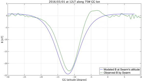
3.2.2 Case 2: March 1, 2016 at 12 p.m. LT

The LT variation of the northward component of a 1-hour magnetic field on the ground for this case study as well as the location information of the ground magnetic data and the Swarm data are illustrated in figure 3.7. The format of the figure is same as that of figure 3.3 except that the data in the figure are from March 1, 2016. The modeled field and the observed field for this case are compared in figure 3.8 in order to confirm whether the modeled field explains or fits the observed values well. The format of this figure is same as that of figure 3.4. In essence, the modeled field corresponds well to the observed-field data points, and therefore, a flow of additional local current is not observed in this case. Figure 3.9 (Figure 3.10) shows the comparison between the estimation of the field (current density) from ground-based data and Swarm-data, just as was shown in figure 3.5 (figure 3.6). The peak amplitudes of both fields are almost comparable, that is, a 1 to 2 nT difference between them is observed. However, the position of the EEJ axis for the ground-based data is shifted southward of the one for the Swarm-based data, i.e. there is a shift from -12.03 degrees of latitude to -11.50 degrees of latitude, respectively. This shift is due to the difficulty involved in determining the zero level of the EEJ-related field, where the mean value from each station during nighttime (6 p.m. to 6 a.m. LT) was used in this study. Another possibility is that local currents could be affecting the profile, that is, decreasing the value obtained at ANC. In addition, it is possible that the peak value was detected at HUA and not at ANC. The estimated current structure from ground magnetic data and Swarm data are shown in figure 3.10. Similarly, the estimated current from the ground data shifts southward of the one estimated from the Swarm data. The peak current densities for the ground-based and Swarm-based estimates were 0.106 A m^-2 and 0.097 A m^-2 respectively.

The widths for the ground-based and Swarm-based estimates were determined as 5.22 degrees of latitude and 4.29 degrees of latitude, respectively. In short, the estimated peak current densities were comparable but a larger amplitude and a southward shift were observed for the estimate from ground-based data when compared to the Swarm-based data.