JAXA Research and Development Report
September 2017
Japan Aerospace Exploration Agency
Pressure Gradient Effects on Mean Flow over Axisymmetric
Bodies at Incidence in Supersonic Flow
- Progress Report of JAXA-NASA Joint Research Project
on Supersonic Boundary Layer Transition (Part 1)
on Supersonic Boundary Layer Transition (Part 1) -
*Hiroaki Ishikawa *1, Naoko Tokugawa *2,
Fei Li *3, Meelan Choudhari *3 and Jeffery White *3
ABSTRACT
Boundary layer transition along the leeward symmetry plane of axisymmetric bodies at zero and non-zero angles of incidence in supersonic flow was investigated numerically as part of joint research between the Japan Aerospace Exploration Agency (JAXA) and National Aeronautics and Space Administration (NASA). Mean flow over five axisymmetric bodies (namely, a Sears-Haack body, a semi-Sears-Haack body, two straight cones and a flared cone) was analyzed to investigate the effects of axial pressure gradient, freestream Mach number, and angle of incidence on boundary layer transition.
Computations revealed the strong effects of axial pressure gradient on boundary layer profile in the vicinity of the leeward symmetry plane, highlighting the three-dimensional dynamics associated with increasing build-up of secondary flow under an adverse axial pressure gradient. Independent flow solutions obtained using different flow solvers and different grids at JAXA and NASA, respectively, were in good agreement with each other. Slight differences between the two sets of solutions are attributed to a combined effect of the differences between respective thermal wall boundary conditions, numerical grids, and flow solvers. The difference due to the thermal boundary condition is confirmed to be physical and was observed for all flow conditions, as expected. However, the other differences were rather minor, and were noticeable only for the straight cone and flared cone configurations. The conditions under which these minor differences are observed and the magnitudes of these differences remain an open question. Despite being coarser than the NASA grids, the JAXA grids are shown to be sufficient for providing basic state definition for the linear stability analysis. Specifically, the results demonstrate that appropriate grid spacing had been used to obtain accurate boundary layer profiles. The present report represents part 1 of a two-part document based on the joint computational effort. Part 1 is devoted to the results of mean flow computations and the results of linear stability analyses and the corresponding experiments are described in part 2.
Keywords: 3-D Boundary Layer, Transition, Computational Fuild Dynamics
doi: 10.20637/JAXA-RR-17-002E/0001
*
Accepted December 8, 2015, Received June 8, 2017
*1
ASIRI Inc.
*2
Aeronautical Technology Directorate, Japan Aerospace Exploration Agency
*3
Contents
Nomenclature··· 4
1 Introduction ··· 5
2 Model Geometry and Flow Conditions ··· 8
3 Computational Methodologies ··· 11
3.1 Numerical Grid ··· 11
3.2 Flow Solvers ··· 13
3.3 Deinition of Boundary Layer Flow Properties ··· 15
4 Results of CFD Analysis at JAXA ··· 17
4.1 Surface Flow Fields ··· 17
4.2 Mean Velocity Proiles ··· 22
4.2.1 Zero incidence coniguration ··· 22
4.2.2 Nonzero incidence coniguration ··· 22
5 Comparison between Computations Based on UPACS and VULCAN Solvers ··· 26
5.1 Thermal Condition Dependency ··· 27
5.2 Grid Dependency··· 29
5.3 Solver Dependency ··· 32
6 Summary ··· 34
Acknowledgments ··· 34
Nomenclature
�� = surface pressure coefficient �� − �∞� �� [1 2⁄ ] �∞�∞2�
� = model length [m]
� = Mach number
� = pressure [Pa]
�(�) = local radius at axial location � [m]
��unit = unit Reynolds number
� = temperature [K]
� = velocity [m/s]
� = axial location with respect to cone apex [m]
� = angle of incidence [deg]
� = boundary layer thickness [mm]
� = cone half-angle [deg]
� = circumferential (i.e., azimuthal) angle with respect to the leeward plane of symmetry [deg]
� = density [kg/m3]
FC = flared cone
max = maximum value
SC = straight cone
SH = Sears-Haack body
SSH = semi-Sears-Haack body
0 = stagnation condition
∞ =
free-stream condition1 Introduction
The Japan Aerospace Exploration Agency (JAXA) and The National Aeronautics and Space
Administration (NASA) have been engaged in joint research on boundary layer transition in
supersonic flow. The objective of the initial research was to improve the knowledge base for
transition mechanisms relevant to the nose region of the fuselage of a supersonic aircraft. To that
end, one of the focal areas for this collaboration was the transition phenomena along the leeward
symmetry plane of axisymmetric bodies at a nonzero angle of incidence.
Although selected portions of the findings from this joint research have already been published
elsewhere [1-3], the detailed results are being documented in two separate reports. In particular, the
present report (part1) is devoted to the computations of the laminar mean flow. The objective
behind these computations is, to pave the way for the investigation, in part 2, of the combined effects
of angle of incidence and axial pressure gradient on boundary layer transition over canonical shapes
of axisymmetric bodies, with an emphasis on transition characteristics near the leeward line of
symmetry. The motivation for this research is described in separate reports [1-3]. However, it is
repeated here in the interest of making this report self-contained.
Drag reduction is one of the most important technical problems that must be addressed to
minimize the fuel burn of transport aircraft, and has been extensively investigated over the years
[4-42]. Despite the potential for viscous drag reduction via increased natural laminar flow (NLF)
over the fuselage, practical application has been rather limited in general and almost nonexistent for
supersonic aircraft [30-41]. A major cause behind the nondeployment of NLF on the fuselage
include the challenges in manufacturing and maintaining sufficiently smooth surfaces. However,
the physical complexity of the transition process over a supersonic fuselage is also a significant
contributor.
The simplest fuselage shape for a supersonic aircraft corresponds to an axisymmetric body.
Transition in boundary layers on axisymmetric bodies in supersonic flow has been extensively
studied in the literature [43-58]. Particularly noteworthy in this context are the tests on a common
5-degree half-angle cone model at zero angle of incidence in various wind tunnel facilities as well as
in flight [49], and the quiet tunnel measurements of a different 5-deg cone model at zero and nonzero
angles of incidence in the Mach 3.5 Supersonic Low Disturbance Tunnel at NASA Langley [50, 51].
Despite the simplicity of the body shape, supersonic flow over a straight cone with circular cross
section is known to exhibit a rich transition behavior. At zero angle of incidence (� = 0 degree), the boundary layer flow is axisymmetric; hence, transition at supersonic free-stream Mach numbers is
dominated by first mode instability. At nonzero angles of incidence, the boundary layer becomes
three dimensional and the inviscid streamlines at the surface become curved due to the azimuthal
pressure gradient from the windward to the leeward side. Therefore, crossflow occurs and the
boundary layer over the side region (i.e., in between the windward and leeward planes of symmetry)
Mach 2, for instance, crossflow transition first occurs at approximately 60 degrees on either side of
the leeward symmetry plane [53]. Even at a finite angle of incidence, supersonic boundary layer
flow along the windward symmetry plane has been shown to exhibit a nearly self-similar behavior
analogous to the case of zero incidence [54] and, furthermore, the instability amplification within
this plane has been shown to remain dominated by first mode instability.
It is well known from the early work on supersonic flow past straight cones [53] that, for
intermediate angles of incidence (up to approximately � �⁄ = 2, where � denotes the angle of incidence and � is the cone half-angle), the boundary layer flow along the leeward plane of symmetry evolves rather differently than elsewhere on the cone surface. Specifically, the
convergence of low-speed secondary flow from both sides of the leeward symmetry plane leads to a
lift-up effect within the plane of symmetry, and hence to a significant thickening of the boundary
layer along the leeward plane. The thicker boundary layer profiles exhibit a strong inflectional
behavior, and hence are more unstable than the boundary layer flow in the adjoining region of the
cone.
Preliminary computations performed at the beginning of this effort showed that the boundary
layer profiles along the leeward symmetry plane are highly sensitive to the magnitude of the axial
pressure gradient. When the pressure gradient along the leeward symmetry plane is favorable, such
as for the flow past the Sears-Haack body at a small angle of incidence, the lift-up effect within the
leeward symmetry plane is substantially reduced. Essentially, the acceleration of the axial velocity
component enables the flow to carry the low-speed fluid converging from both sides of the leeward
plane. Consequently, the velocity profiles along the leeward symmetry plane can remain
noninflectional over longer distances, resulting in a more stable boundary layer flow. This alters the
relative locations of transition location along the leeward plane and the earliest location of
crossflow-induced transition over the side of the cone. Indeed, major changes in the transition front
characteristics can occur as the body shape is varied. An understanding of these changes is relevant
to the aerodynamic design of an aircraft nose targeting a longer region of NLF.
Transition fronts with three local minima, one along the leeward symmetry plane and one each
due to crossflow transition on either side have previously been observed and/or predicted in the
context of straight cones [51-54] and a delta wing configuration [55]. However, the physics of
transition along the leeward plane and the effect of axial pressure gradient on the corresponding
transition location has not been scrutinized in detail, perhaps due to the narrow width of the
transition lobe centered on the leeward symmetry plane and/or the reduced wall shear stress
associated with the thicker boundary layer in that region. The latter factors aside, the ubiquitous
nature of analogous transition patterns in the context of fully 3D high-speed flows over slender
bodies [56, 57]makes it even more useful to examine the transition process along the leeward
The following section introduces the five different axisymmetric bodies with varying axial
pressure gradients, which were used during the present investigation. Computational Methodologies
are described in Section 3. The results of JAXA are described in Section 4. More in-depth
comparison between the results of JAXA and NASA is discussed in Section 5. A summary of the
2 Model Geometry and Flow Conditions
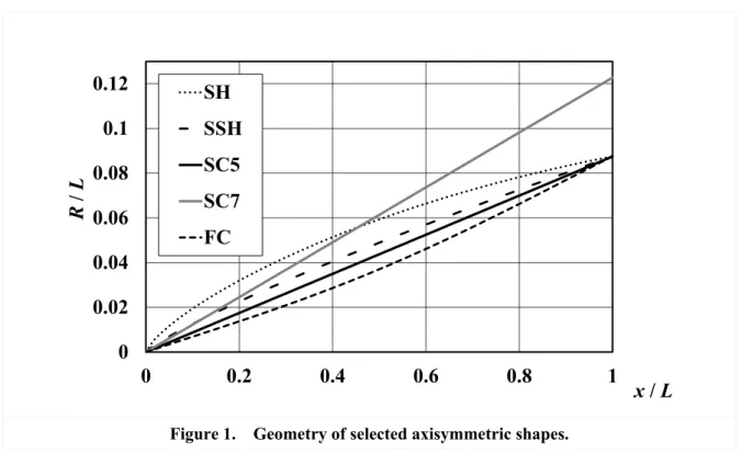
The five different axisymmetric bodies targeted in the present investigation are the Sears-Haack
body, a semi-Sears-Haack body, two straight cones, and a flared cone. The shapes of all five bodies
are plotted in Fig. 1, wherein � denotes the axial coordinate relative to the cone apex and � represents the local body radius at a given station. � denotes the azimuthal directions. �= 0 degree corresponds to the leeward symmetry plane, and �= 180 degree corresponds to the windward symmetry plane.
The model length in axial direction � is taken as �= 0.33 m, similar to that in the experiments.
Figure 1. Geometry of selected axisymmetric shapes.
The Sears-Haack body (abbreviated as SH in the following) produces the least wave drag for a
given length and maximum diameter based on slender body theory (i.e., solution of the linearized
potential equation). Its shape is defined by the following expression for the axial distribution of
local body radius�SH(�):
�SH(�) =�0[(� �⁄ SH){1−(� �⁄ SH)}]�3 4� � , (1) where �SH(�) = 1.194938 m and �0(�) = 0.09657 m. However, the object of analysis is the nose part of it with a length of �= 0.33 m.
The semi-Sears-Haack body (abbreviated as SSH in the following) corresponds to a linearly
weighted mean of the radius distributions for the Sears-Haack body and straight cone, as expressed
by the radius distribution�SSH(�):
�SSH(�) = 0.3 �SH(�) + 0.7 �SC(�), (2)
0
0.02
0.04
0.06
0.08
0.1
0.12
0
0.2
0.4
0.6
0.8
1
R
/
L
x
/
L
SH
SSH
SC5
SC7
FC
� � � � � � � � � �−−9�4 −7�3− −5�2 −2� − −4
where �SC(�) corresponds to the local radius of the straight cone as defined below. It was intended to model the effects of a weak but favorable axial pressure gradient, i.e., a pressure gradient
that is intermediate to the modestly favorable gradient along the SH body and the near-zero gradient
on the straight cone. The precise choice of the weighting coefficients was somewhat arbitrary, but
was justified via linear stability calculations that established visible differences in linear
amplification characteristics from the other two cases.
The straight cone geometry is defined by the cone half-angle, which is equal to 5 degrees or 7
degrees for the present study. The variation of model radius with the axial coordinate is defined as
follows:
�SC(�) = � tan�. (3)
The straight cones are collectively denoted as SC, and the SC configurations with a half angle � of 5 degrees and 7 degrees are individually abbreviated as SC5 and SC7, respectively.
Finally, the flared cone (abbreviated as FC in the following) geometry is defined by the following
distribution of model radius:
�FC(�) =
�−1.0478 × 10
−9�4+ 6.9293 × 10⁻⁷�3−6.1497 × 10⁻⁵�2+ 6.998 × 10⁻²� −6.2485 × 10⁻⁴
0
(4)
where the axial coordinate x is measured in meters.
The semi-Sears-Haack body and the flared cone configuration were originally designed in JAXA
for investigating the influence of pressure gradient on the flow characteristics near the leeward
symmetry plane [58]. As mentioned in the Introduction, the effects of secondary flow convergence
from both sides of the leeward symmetry plane and the associated lift-up of low-speed fluid away
from the surface are expected to increase as the axial flow along this plane goes from accelerated
(SH, SSH) to nearly constant velocity along the cone axis (SC5 and SC7) to decelerated (FC).
Table 1 provides the summary of studied cases as well as introducing a composite notation that
combines the information about the shape, angle of incidence, and stagnation pressure. For example,
the case SC5-0deg-99 from Table 1 refers to the straight cone with 5-degree half angle SC at
0-degree incidence and a stagnation pressure of 99 kPa.
The quantities �∞,�0,�∞, and ��unit denote the Mach number, stagnation pressure, static temperature, and unit Reynolds number, respectively, of the oncoming freestream. The flow
conditions from Table 1 correspond to the nominal values during a series of experiments. With the
Low Disturbance Tunnel at NASA Langley Research Center, the flow conditions for all other bodies
correspond to the experiments conducted by JAXA.
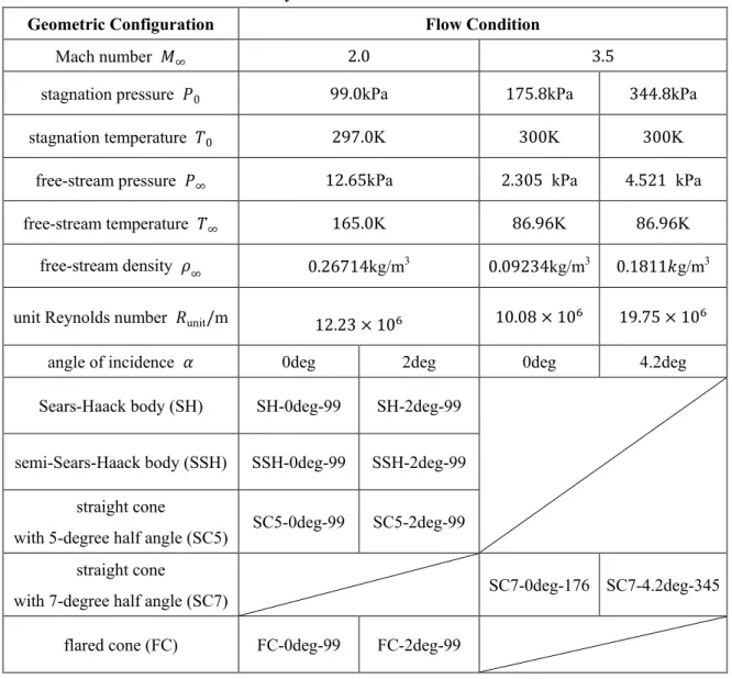
Table 1: Summary of flow conditions and case notation.
Geometric Configuration Flow Condition
Mach number �∞ 2.0 3.5
stagnation pressure �0 99.0kPa 175.8kPa 344.8kPa
stagnation temperature �0 297.0K 300K 300K
free-stream pressure �∞ 12.65kPa 2.305 kPa 4.521 kPa
free-stream temperature �∞ 165.0K 86.96K 86.96K
free-stream density �∞ 0.26714kg/m3 0.09234kg/m3 0.1811�g/m3
unit Reynolds number �unit/m 12.23 × 10⁶ 10.08 × 10⁶ 19.75 × 10⁶
angle of incidence � 0deg 2deg 0deg 4.2deg
Sears-Haack body (SH) SH-0deg-99 SH-2deg-99
semi-Sears-Haack body (SSH) SSH-0deg-99 SSH-2deg-99
straight cone
with 5-degree half angle (SC5) SC5-0deg-99 SC5-2deg-99
straight cone
with 7-degree half angle (SC7) SC7-0deg-176 SC7-4.2deg-345
flared cone (FC) FC-0deg-99 FC-2deg-99
3 Computational Methodologies
3.1 Numerical Grid
Mean-flow computations are conducted using two different numerical grids, which were
independently generated based on their own knowledge and experience by JAXA and NASA,
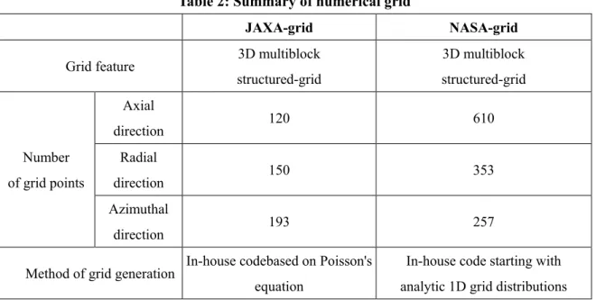
respectively. The salient features of both grids are summarized in Table 2.
Table 2: Summary of numerical grid
JAXA-grid NASA-grid
Grid feature 3D multiblock structured-grid
3D multiblock
structured-grid
Number
of grid points
Axial
direction 120 610
Radial
direction 150 353
Azimuthal
direction 193 257
Method of grid generation In-house codebased on Poisson's equation
In-house code starting with
analytic 1D grid distributions
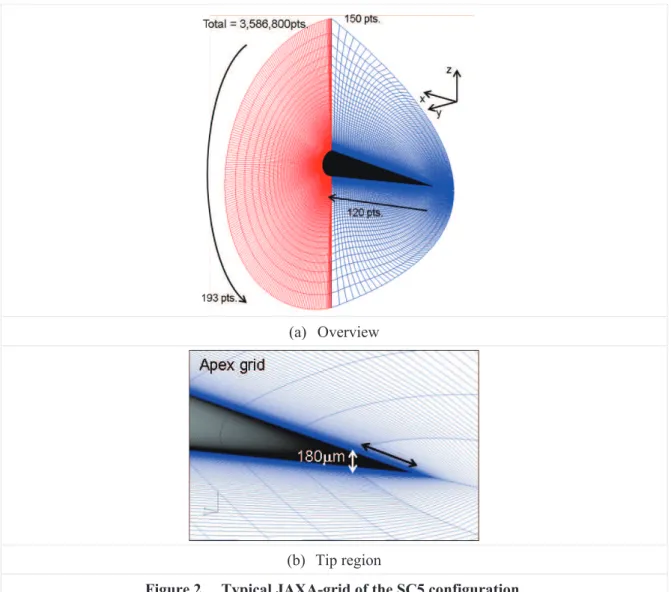
The grid generated by use of a JAXA in-house code (abbreviated as JAXA-grid in the following)
was a 3-dimensional multi-structured grid. And it is used for the mean flow computation at JAXA. It
has a typical grid size of 120 points in the axial direction, 150 points in the surface normal direction,
and more than 193 points in the azimuthal (i.e., circumferential) direction, with a total of 3,586,800
grid points.
A typical JAXA grid is shown in Figures 2(a) and 2(b). As shown in the figures, the grid spacing
is gradually stretched in the axial direction using the tangent and hyperbolic tangent function
suggested by Vinokur [59]. The nose is assumed to be sharp with zero radius. The axial spacing
near the tip is about 1000 μm at the axial location where the cone diameter becomes 180 μm (Fig.
2(b)). The axial spacing at the downstream end of the cone is approximately 8.8 mm
The azimuthal grid is equispaced at every 1 deg, except for narrow regions near the leeward and
windward symmetrical planes where the azimuthal spacing decreases to 0.11 deg in order to capture
the flow details near the attachment line (windward plane) and those associated with the
convergence of the secondary flow (near the leeward ray). The radial, i.e., wall-normal grid is
generated via the solution of an elliptic partial differential equation (Poisson’s equation) suggested
by Thompson [60] and Steger-Sorenson’s method [61]. The outer edge of the grid within the
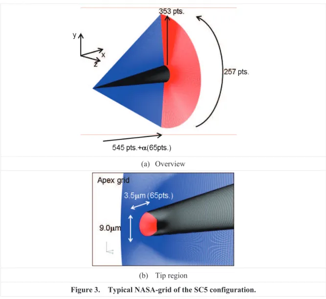
A typical NASA grid is shown in Fig. 3. It has 610 points in the axial direction, 353 points in the
surface normal direction, and more than 257 points in the azimuthal direction, with a total of
52,765,734 points.
As shown in Fig. 3, the grid spacing is gradually stretched in the axial direction, analogous to the
JAXA grid described previously. However, the NASA grid is distributed much more densely at the
tip region in comparison with the JAXA grid. The nose radius was assumed to be nonzero but tiny.
The radius of approximately 3.5μm was resolved with approximately 65 axial points and the shock
layer in front of it was captured within the computational domain. The number of grid points
between the tip and the downstream end of the cone is 545, which is also larger than the
corresponding number of grid points in the JAXA grid. The azimuthal grid has similar characteristics
as the JAXA grid, i.e., it is equally spaced except in a narrow region near the leeward and windward
symmetry planes. The azimuthal grid near the leeward symmetry plane is nearly five times denser
than that in the remaining region. The wall-normal grid distribution was different from that in the
(a) Overview
(b) Tip region
JAXA grid. The NASA grid is distributed equally across the boundary layer, and the grid begins to
stretch only after the radial location is well outside of the edge of the boundary layer. The outer edge
of the grid within the symmetry plane is again C-shaped, similar to the JAXA grid.
(a) Overview
(b) Tip region
Figure 3. Typical NASA-grid of the SC5 configuration.
3.2 Flow Solvers
Two different flow solvers were used for this purpose and extensive comparisons were made
between the respective solutions to ensure that the computed mean flow solutions were independent
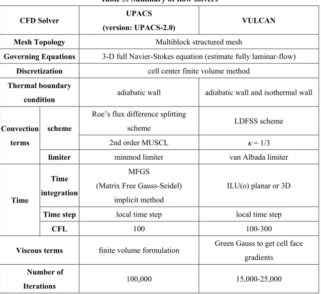
of the code. The relevant features of both codes are summarized in Table 3.
Computations with adiabatic thermal wall boundary conditions were performed using the 3D,
multiblock, structured-grid flow solver UPACS (Unified Platform for Aerospace Computational
Simulation) [62] that was developed at JAXA.
Independent computations for the same test conditions were performed at NASA using an
analogous 3D, multiblock, structured-grid flow solver, VULCAN [63], which was developed at the
compute the basic state solutions corresponding to the isothermal wall boundary condition (�w = 300 K).
The laminar basic state at each condition was obtained using numerical solutions to the
compressible Navier-Stokes equations. An isothermal boundary condition is more appropriate for
the short duration tests corresponding to a higher stagnation pressure (�0 = 99 kPa) in FWT, the 0.6m×0.6m High Speed Wind Tunnel at Fuji Heavy Industries in Japan. In this case, the surface
temperature of the model was set to �w = 300 K. For the FWT test conditions, the estimated recovery temperature (based on a recovery factor of 0.85) is 277 K. Thus, the isothermal model
temperature of �w = 300 K corresponds to �w⁄�ad≈1.08.
Table 3: Summary of flow solvers
CFD Solver
UPACS
(version: UPACS-2.0) VULCAN
Mesh Topology Multiblock structured mesh
Governing Equations 3-D full Navier-Stokes equation (estimate fully laminar-flow)
Discretization cell center finite volume method
Thermal boundary
condition
adiabatic wall adiabatic wall and isothermal wall
Convection
terms
scheme
Roe’s flux difference splitting
scheme
LDFSS scheme
2nd order MUSCL κ = 1/3
limiter minmod limiter van Albada limiter
Time
Time
integration
MFGS
(Matrix Free Gauss-Seidel)
implicit method
ILU(o) planar or 3D
Time step local time step local time step
CFL 100 100-300
Viscous terms finite volume formulation Green Gauss to get cell face
gradients
Number of
Iterations
100,000 15,000-25,000
Solutions on multiple grids with different grid counts were compared to ensure that the computed
laminar state was insensitive to the grid resolution. To establish the grid convergence of the basic
state solutions in a definitive manner, the VULCAN computations used a wider range of grid sizes.
In order to provide sufficiently accurate description of the basic state for linear stability analysis, the
δ
� �� ��⁄ � � �� ��⁄
��1 �
�� �2 ��
�� �3 ��
�1
�2 ��1
�� �2 �3 �
� �� ��⁄ �
δ
UPACS grids had at least 50 to 80 grid points in the boundary layer and more than 80 points in the
case of the VULCAN solutions. This type of wall-normal resolution had been found to be sufficient
for linear stability analysis in a related study conducted previously. The azimuthal grids were
clustered near the leeward symmetry plane in order to capture the potential influence of azimuthal
diffusion on the boundary layer flow in the vicinity of the symmetry plane.
3.3 Definition of Boundary Layer Flow Properties
As part of post processing from the computed mean flow solutions, the boundary layer thickness
was computed by defining the boundary layer edge as the wall-normal distance δ such that:
[�(��)⁄��]�= 0.01 × [�(��)⁄��]wall. (5)
In order to find the most suitable definition of boundary layer edge, other definitions were also
examined, namely,
��1= 0.99 �max, (6)
[��]�2= 0.99 × [��]max, (7)
[��]�3 = 0.999 × [��]max. (8)
The values of boundary layer thickness based on these definitions are compared in Figure 4. �1 and �2 are thinner than the other predicted thickness values. Thus, the definitions based on ��1 and [��]�2 were not adopted. On the other hand, �3is very close to �. Near the nose vertex, it is difficult to capture the boundary layer edge because of the interference of the shock wave from the
nose vertex. However, the definition based on eq. (5) is based on the surface physical values and
independent of the shock wave from the nose vertex. Hence, [�(��)⁄��]� was adopted in the definition of the boundary layer edge in this study.
(a) Boundary Layer Thickness (b) Boundary Layer on the Straight Cone
Figure 4. Definition of Boundary Layer Edge (SC5-2deg-99).
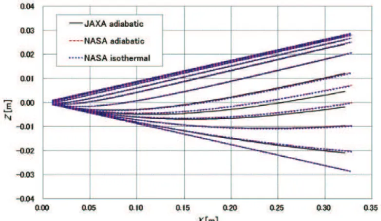
The inviscid streamlines are extracted based on the flow properties corresponding to the selected
definition of the boundary layer edge. Linear interpolation was used to obtain flow properties in
0.0000 0.0001 0.0002 0.0003 0.0004 0.0005 0.0006 0.0007
0.00 0.05 0.10 0.15 0.20 0.25 0.30 0.35
δ
(m)
X (m)
Umax*99% (rho*U)max*99% (rho*U)max*99.9% d(rho*U)/dy*1% 0.0000 0.0005 0.0010 0.0015 0.0020 0.0025 0.0030 0.0035 0.0040
0.00 0.01 0.02 0.03 0.04
R
+δ
(m)
X (m)
between computational grid points neighboring the points on the inviscid streamlines (Figure 5). The
extracted external streamline is illustrated in Figure 6.
Figure 5. Illustration of Extraction of External Streamlines.
Figure 6. Extracted External Streamlines (SC5-2deg-99).
External stream line
Integral path for the Transition analysis Velocity vector
Start point is given by grid index
4 Results of CFD Analysis at JAXA
The results of mean flow computation based on JAXA’s UPACS flow solver in conjunction with
an adiabatic thermal boundary condition are described in this section.
4.1 Surface Flow Fields
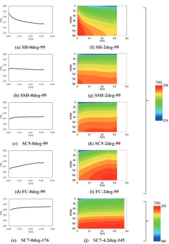
Figures 7(a) through 7(e) display the axial variation in surface pressure coefficient for each of the
five body shapes at zero-degrees angle of incidence. Figures 7(f) through 7(j) display the contours of
surface pressure coefficient for each of the five body shapes at nonzero degrees angles of incidence,
where the flow field becomes nonaxisymmetric and the surface pressure depends on both axial and
azimuthal coordinates.
The results in Fig. 7 indicate that the pressure gradient in the axial direction varies with the body
shapes. As alluded to previously, it is favorable along the SH and SSH body shapes, but almost zero
for the SC5, SC7 and adverse for the FC. The favorable pressure gradient along the length of the
SSH body is weaker in comparison with that along the SH body. This qualitative behavior is
Regardless of the body shape, however, there is always a positive azimuthal pressure gradient at
any fixed axial station when the bodies are placed at a nonzero angle of incidence. This azimuthal
(a) SH-0deg-99 (f) SH-2deg-99
(b) SSH-0deg-99 (g) SSH-2deg-99
(c) SC5-0deg-99 (h) SC5-2deg-99
(d) FC-0deg-99 (i) FC-2deg-99
(e) SC7-0deg-176 (j) SC7-4.2deg-345
Figure 7. Surface pressure distribution [1-4].
0.1
0.0 Cp
0.06
0.00 Cp Cp
pressure gradient drives a circumferential flow from the windward to the leeward side, and hence,
causes the boundary layer flow to become fully three-dimensional.
Figure 8 displays the contours of surface temperature distribution.
(a) SH-0deg-99 (f) SH-2deg-99
(b) SSH-0deg-99 (g) SSH-2deg-99
(c) SC5-0deg-99 (h) SC5-2deg-99
(d) FC-0deg-99 (i) FC-2deg-99
(e) SC7-0deg-176 (j) SC7-4.2deg-345
Figure 8. Surface temperature distribution at zero and nonzero angles of incidence and
adiabatic thermal boundary condition. 275 276 277 278 279 280
0.00 0.10 0.20 0.30 0.40
T [K ] X[m] 275 276 277 278 279 280
0.00 0.10 0.20 0.30 0.40
T [K ] X[m] 275 276 277 278 279 280
0.00 0.10 0.20 0.30 0.40
T [K ] X[m] 275 276 277 278 279 280
0.00 0.10 0.20 0.30 0.40
T [K ] X[m] 265 266 267 268 269 270
0.00 0.10 0.20 0.30 0.40
T
[K
]
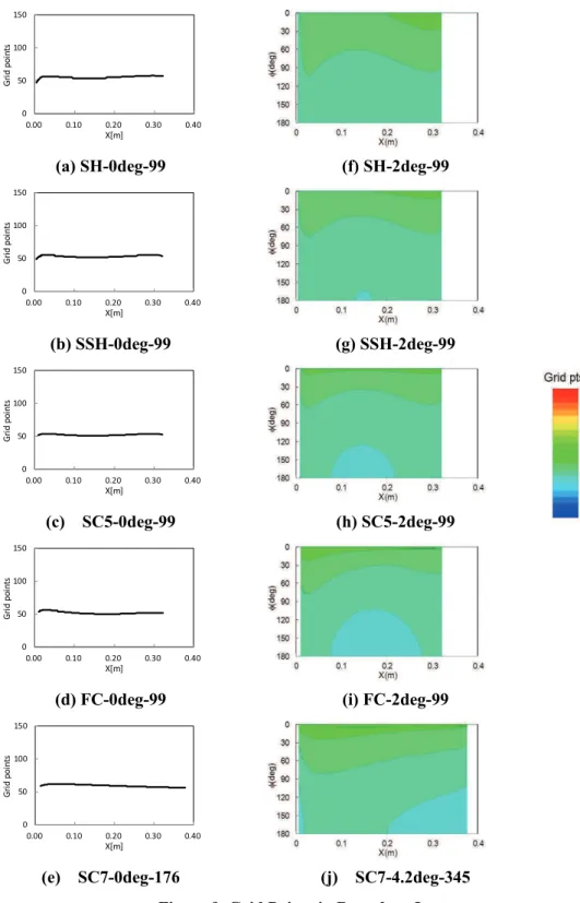
Figure 9 indicates that the number of grid points across the boundary layer is more than 50, but
less than 70. As described below, although this number is smaller than that corresponding to the
denser grids employed at NASA, it is nonetheless sufficient to provide an accurate basic state
definition for linear stability analysis (see subsection 5.2 and 5.3).
(a) SH-0deg-99 (f) SH-2deg-99
(b) SSH-0deg-99 (g) SSH-2deg-99
(c) SC5-0deg-99 (h) SC5-2deg-99
(d) FC-0deg-99 (i) FC-2deg-99
(e) SC7-0deg-176 (j) SC7-4.2deg-345
Figure 9. Grid Points in Boundary Layer.
0 50 100 150
0.00 0.10 0.20 0.30 0.40
G ri d po int s X[m] 0 50 100 150
0.00 0.10 0.20 0.30 0.40
G ri d po int s X[m] 0 50 100 150
0.00 0.10 0.20 0.30 0.40
G ri d po int s X[m] 0 50 100 150
0.00 0.10 0.20 0.30 0.40
G ri d po int s X[m] 0 50 100 150
0.00 0.10 0.20 0.30 0.40
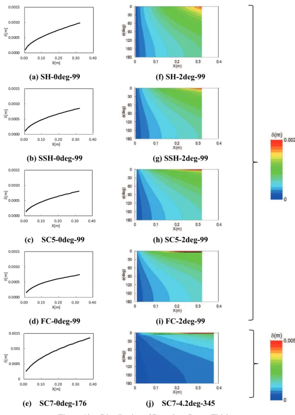
Figure 10 displays the distribution of boundary layer thickness for the flow configurations of
interest. Contrary to the surface pressure and surface temperature distributions, the pattern of
boundary layer thickness distributions remains similar for all flow configurations.
(a) SH-0deg-99 (f) SH-2deg-99
(b) SSH-0deg-99 (g) SSH-2deg-99
(c) SC5-0deg-99 (h) SC5-2deg-99
(d) FC-0deg-99 (i) FC-2deg-99
(e) SC7-0deg-176 (j) SC7-4.2deg-345
Figure 10. Distribution of Boundary Layer Thickness.
0.0000 0.0005 0.0010 0.0015
0.00 0.10 0.20 0.30 0.40
δ[ m ] X[m] 0.0000 0.0005 0.0010 0.0015
0.00 0.10 0.20 0.30 0.40
δ[ m ] X[m] 0.0000 0.0005 0.0010 0.0015
0.00 0.10 0.20 0.30 0.40
δ[ m ] X[m] 0.0000 0.0005 0.0010 0.0015
0.00 0.10 0.20 0.30 0.40
δ[ m ] X[m] 0 0.0005 0.001 0.0015
0.00 0.10 0.20 0.30 0.40
δ[
m
]
4.2 Mean Velocity Profiles
4.2.1 Zero incidence configuration
The axial development of the mean velocity profiles along a generatrix at zero-degrees angle of
incidence is shown in Figs. 11(a) through 11(e). For the purpose of comparison, velocity profiles for
the axisymmetric flow over five kinds of bodies are shown in each figure. The sets of profiles are
virtually self-similar as seen from the collapse of all three curves in each figures.
(a) SH-0deg-99
(b) SSH-0deg-99
(c) SC5-0deg-99
(d) FC-0deg-99
(e) SC7-0deg-176
Figure 11. Mean velocity profiles on the zero incidence configurations.
4.2.2 Nonzero incidence configuration
The mean velocity profiles, along the windward and the leeward symmetry planes for a nonzero
angle of incidence are shown in Figs. 12 and 13, respectively.
(a) SH-0deg-99
(b) SSH-0deg-99
(c) SC5-0deg-99
(d) FC-0deg-99
(e) SC7-0deg-176
As shown in Fig. 12, the mean velocity profiles along the windward symmetry plane are
self-similar, analogous to the zero incidence configurations. The flow in the vicinity of the windward
symmetry plane diverges from the symmetry plane to both sides. This character of the flow is
independent of the axial pressure gradient, and hence, remains the same for all body shapes.
(a) SH-2deg-99 (a) SH-2deg-99
(b) SSH-2deg-99 (b) SSH-2deg-99
(c) SC5-2deg-99 (c) SC5-2deg-99
(d) FC-2deg-99 (d) FC-2deg-99
(e) SC7-4.2deg-345 (e) SC7-4.2deg-345
Figure 12. Mean velocity profiles along the
windward symmetry plane at incidence.
Figure 13. Mean velocity profiles along the
leeward symmetry plane at incidence.
(a) SH-2deg-99 (a) SH-2deg-99
(b) SSH-2deg-99 (b) SSH-2deg-99
(c) SC5-2deg-99 (c) SC5-2deg-99
(d) FC-2deg-99 (d) FC-2deg-99
(e) SC7-4.2deg-345 (e) SC7-4.2deg-345
In contrast to the zero incidence configuration as well as to the flow along the windward
symmetry plane, the boundary layer flow near the leeward plane has a strong dependence on the
body shape as shown in Figs. 13(a) through 13(e). As shown in Fig. 13(a), in the SH-2deg-99 case,
the flow continues to develop in the axial direction and is not self-similar. The variation in velocity
profiles over the same range of locations becomes stronger as the magnitude of the favorable
pressure gradient in the axial direction is reduced from the SH body shape (Fig. 13(a)) to the SSH
body shape (Fig. 13(b)). The largest velocity profile variation on the SSH body occurs near the tip
where the axial pressure gradient is strong. However, the velocity profile variation remains strong,
even at the aft of the body, where the axial pressure gradient becomes weaker. These observations
indicate that the velocity profile variation is not determined by the axial pressure gradient alone. The
azimuthal pressure gradient also has a major influence on the secondary flow that converges along
the leeward symmetry plane and, in turn, exerts a significant influence on the thickening of the
boundary layer.
The velocity profiles in the axisymmetric case (SC5-0deg-99) remain noninflectional at all
stations (Fig. 11(a)). However, due to an increase in density away from the wall, the density
weighted shear (or, equivalently, angular momentum) profile ��� ⁄ �� achieves its maximum inside the boundary layer. From the comparison of ��� ⁄ �� profiles, the existence of a generalized inflection point was found to imply that the boundary layer supports an inviscid
instability mechanism in addition to the viscous-inviscid interactive Tollmien-Schlichting modes that
exist even in the absence of the inflection point [3]. A comparison of ��� ⁄ �� profiles for the SC5-0deg-99 and the SC5-2deg-99 cases revealed that the interior peak becomes stronger in the
latter case, especially at larger�, indicating a stronger inviscid instability along the leeward plane. The generalized inflectional behavior of the leeward profiles becomes even more prominent in the
adverse pressure gradient case (FC-2deg-99) and progressively weakens when the axial pressure
gradient becomes increasingly favorable (i.e., SSH-2deg-99 and SH-2deg-99 cases). These trends in
inflectional behavior are correlated with the increasingly stronger instability along the leeward
symmetry plane as the body shape varies from SH to FC [3]. The trends in generalized inflection
characteristics with respect to both � and the axial pressure gradient are also correlated in part with the inflectional behavior of the velocity profiles. For instance, the existence of inflection in the
SC5-2deg-99 case is clearly seen from the velocity profiles in Fig. 13(c) and the inflection becomes
stronger when the axial pressure gradient becomes positive (case FC-2deg-99 in Fig. 13(d)). In fact,
at � = 300 mm in the FC-2deg-99 case, the region of highest velocity gradient across the boundary layer has lifted away from the surface, closer to the edge of the boundary-layer. Of course, such
boundary layer lift up is unlikely to be observed in practice, because the strong inflectional
instability of the leeward boundary layer should cause laminar-turbulent transition ahead of this
As already mentioned above, the convergence of low-speed secondary flow from both sides of the
leeward symmetry plane leads to a lift-up effect within the plane of symmetry, and hence, to a
significant thickening of the boundary layer along the leeward plane. The thicker boundary layer
profiles exhibit a strongly inflectional behavior, and hence are more unstable than the boundary layer
flow at adjoining locations away from the region of boundary layer thickening near the leeward
plane. This lift-up effect becomes stronger as the deceleration, due to the adverse pressure gradient
along the leeward symmetry plane, becomes stronger. The lift-up effect eventually results in a
“mushroom”-like flow pattern around the leeward symmetry plane as shown in the velocity contours
in Fig. 14. It is obvious that the size of the “mushroom” structure is strongly dependent on the
(a) SH-2deg-99
(b) SSH-2deg-99
(c) SC5-2deg-99
(d) FC-2deg-99
(e) SC7-4.2deg-345
Figure 14. Mean velocity distribution near leeward plane of symmetry (x = 0.25 m).
5 Comparison between Computations Based on UPACS and VULCAN Solvers
The laminar basic states computed with the UPACS and VULCAN flow solvers were compared
with each other to establish that the boundary layer profiles used for stability analysis were
independent of the flow solver and the grid topology used.
(a) SH-2deg-99
(b) SSH-2deg-99
(c) SC5-2deg-99
(d) FC-2deg-99
(e) SC7-4.2deg-345
5.1 Thermal Condition Dependency
The flow characteristics obtained via the VULCAN flow solver were compared with those
obtained by UPACS, using the SC5-0deg-99 case as an example. The results are shown in Fig. 15
through Fig. 19. The results of UPACS, which were already shown in the previous section, are
duplicated herein to allow a side-by-side comparison.
This subsection is devoted to the effects of the thermal boundary condition, since only an
adiabatic solution could be obtained via the UPACS solver, but both adiabatic and isothermal cases
could be addressed using VULCAN as described previously.
(a) UPACS (adiabatic) (Fig. 7 (h)) (a) UPACS (adiabatic) (Fig. 8 (h))
(b) VULCAN (adiabatic) (b) VULCAN (adiabatic)
(c) VULCAN (isothermal) (c) VULCAN (isothermal)
Figure 15. Comparison of surface pressure
distribution between UPACS and VULCAN for
flow configuration SC5-2deg-99.
Figure 16. Comparison of surface temperature
distribution between UPACS and VULCAN for
flow configuration SC5-2deg-99.
As shown in the figures, both results of VULCAN are in reasonable agreement with the
corresponding UPACS solutions. In particular, the surface pressure distributions in Fig. 15, and the
boundary layer thickness in Fig. 18, indicate good agreement amongst all three computation. On the
other hand, the surface temperature distributions, which are shown in Fig. 16, and the number of grid
points across the boundary layer, which are shown in Fig. 17, indicate expected differences. The
surface temperature distributions for adiabatic cases are in good agreement, but those obviously
across the boundary layer are much smaller than that in the both of the VULCAN cases, but that was
expected because of the differences in the numerical grids. Although omitted from this paper, other
quantities at the boundary layer edge, such as the edge pressure and edge density distribution along
the body length are also in good agreement among the three solutions (namely, the adiabatic case
with UPACS and VULCAN, and the isothermal case with VULCAN).
(a) UPACS (adiabatic) (Fig. 9 (h)) (a) UPACS (adiabatic) (Fig. 10 (h))
(b) VULCAN (adiabatic) (b) VULCAN (adiabatic)
(c) VULCAN (isothermal) (c) VULCAN (isothermal)
Figure 17. Comparison of Grid Points in
Boundary Layer between UPACS and
VULCAN on SC5-2deg-99.
Figure 18. Comparison of Boundary Layer
Thickness between UPACS and VULCAN on
SC5-2deg-99.
The wall-normal profiles of axial velocity based on all three solutions show relatively small
differences (Fig. 19). Even smaller differences are seen between the velocity profiles based on the
UPACS and VULCAN solutions for an adiabatic wall. Since grid convergence of the VULCAN
solutions had been established, these very small differences between the VULCAN and UPACS
solutions for an adiabatic wall are attributed to slight shortcomings of grid resolution in the UPACS
solution as shown below; furthermore, these differences were noticeable only in the vicinity of the
(a) UPACS (adiabatic) (Fig. 14 (c))
(b) VULCAN (adiabatic)
(c) VULCAN (isothermal)
Figure 19. Comparison of axial velocity profiles along the leeward symmetry
plane between UPACS and VULCAN solutions for SC5-2deg-99.
5.2 Grid Dependency
Next, we turn our attention to the differences between the results of UPACS-adiabatic and
VULCAN-adiabatic cases (i.e., on the effects of computational process alone, with the same
physical boundary conditions). The profiles of axial velocity and temperature based on the two sets
of solutions are compared with each other in Figs. 20 and 21, respectively. The isothermal
solutions are also plotted as a reference.
As already mentioned in the previous subsection, the differences between the two adiabatic
solutions are relatively small and are confined to the axial velocity profile along the leeward
symmetry plane (Fig. 20(a)).
Similar differences are observed along the leeward symmetry plane of the flared-cone
(FC-2deg-99) and the limited tip side area of the flared-cone (FC-2deg-99). In other words, the
differences along the windward symmetry plane, or on the semi-Sears-Haack (SSH-2deg-99) and the
Sears-Haack (SH-2deg-99) bodies are relatively insignificant, i.e., comparable to the expected
(a) Along leeward symmetry plane (� = 0 º) (a) Along leeward symmetry plane (� = 0 º)
(b) Along the side (� = 90 º) (b) Along the side (� = 90 º)
(c) Along windward symmetry plane (� = 180 º) (c) Along windward symmetry plane (� = 180 º)
Figure 20. Comparison of axial velocity
profiles from UPACS and VULCAN
solutions for SC5-2deg-99 at � = 300 mm.
Figure 21. Comparison of temperature profiles
from UPACS and VULCAN solutions for
SC5-2deg-99 at � = 300 mm.
The small differences between the two adiabatic computations is attributed to the difference
between grid resolution and/or the difference between flow solvers. To help clarify the origin of this
discrepancy, the NASA grid is used with the UPACS solver to obtain the mean flow for the
SC5-2deg-99 case. Figs. 22 and 23 compare the results with the original solutions based on different
grids, i.e., UPACS solution using the JAXA grid and VULCAN solution using the NASA grid. The
boundary layer profiles along the leeward plane are compared in Fig. 24. The UPACS solutions
using the NASA grid are in better agreement with the VULCAN solutions using the same grid. This
comparison shows that UPACS and VULCAN are able to obtain nearly the same results when the
same computational mesh is used. On the other hand, UPACS solutions for different grid
distributions indicate small discrepancies along the leeward symmetry plane of the SC5-2deg-99
configuration. Thus, the origin of the differences between the UPACS and VULCAN solutions is
attributed to modest grid dependency of the UPACS solution. However, these differences associated � �
(a) Along leeward symmetry plane (� = 0 º) (a) Along leeward symmetry plane (� = 0 º)
(b) Along the side (� = 90 º) (b) Along the side (� = 90 º)
� �
with grid resolution do not have a noticeable impact on the predicted transition locations as
demonstrated in Refs. 1-3.
(a) UPACS on JAXA-grid
(Fig. 17 (a))
(a) UPACS on JAXA-grid
(Fig. 18(a))
(b) UPACS on NASA-grid (b) UPACS on NASA-grid
(c) VULCAN on NASA-grid
(Fig. 17 (b))
(c) VULCAN on NASA-grid
(Fig. 18 (b))
Figure 22. Comparison of surface
temperature distribution for SC5-2deg-99.
Figure 23. Comparison of number of grid
points across boundary layer for SC5-2deg-99.
(a) axial velocity profiles (b) temperature profiles
Figure 24. Comparison of boundary layer profiles based on UPACS and VULCAN
A Similar comparison is conducted for the flared-cone (FC-2deg-99). In this case, the UPACS
solutions using the NASA grid does not bring the improved agreement that was observed earlier for
the straight cone case. As shown in Fig. 25(c), the UPACS solution using the NASA grid leads to
improved agreement with the VULCAN solution for the axial velocity profile at � = 50 mm along the side of the cone (� = 90º). Since the differences among the three profiles at � = 300 mm along the side of the cone are negligible in magnitude (Fig. 25(d)), the difference at � = 50 mm is likely to have been caused by grid difference and the higher sensitivity of the boundary layer profiles at
that location to the difference in computational grid near the cone tip.
Along the leeward symmetry plane (� = 0º) at x = 300 mm, using the same grid actually results in a larger difference between the two profiles (Fig. 25 (b)). Similarly, near the tip at � = 50 mm, the difference becomes larger as well (Fig. 25 (a)). The original difference between the UPACS solution
using the JAXA grid and the VULCAN solution using the NASA grid was very small. But the
difference between the UPACS and VULCAN solutions using the NASA grid is larger than that
observed with the original grids.
(a) � = 50mm, along leeward symmetry
plane (� = 0 º)
(b) � = 300 mm, along leeward symmetry
plane (� = 0 º)
(c) � = 50mm, at side region (� = 90 º) (d) � = 300mm, at side region (� = 90 º)
Figure 25. Comparison of axial velocity profiles between UPACS and VULCAN
solutions for FC-2deg-99.
5.3 Solver Dependency
Since there are differences in UPACS and VULCAN solutions along the leeward symmetry plane
of the flared-cone (FC-2deg-99) even when the same grid is used, those differences are presumably
caused by the differences in the underlying numerical algorithms. Therefore, some of the numerical
�
�
�
�
�
� �
�
�
�
(a) � = 50mm, along leeward symmetry
plane (� = 0 º)
(b) � = 300 mm, along leeward symmetry
plane (� = 0 º)
parameters in the UPACS solution were adjusted in order to reduce the differences between the
respective algorithms. In particular, the role of the difference between the respective limiter
functions (“minmod limiter” in UPACS calculation versus “van Albada limiter” in VULCAN
computation as shown in Table 3) was assessed.
Therefore, the UPACS solution was recomputed by using the “van Albada limiter” similar to the
VULCAN computation. The results in Fig. 26 confirm that the profiles obtained by UPACS with the
“van Albada limiter” (shown at the green line in Fig. 26) move closer to the profiles obtained by
VULCAN using the same limiter (shown at the red line in Fig. 26) in comparison with the profiles
obtained by UPACS with “minmod limiter” (shown at the blue lines in Fig. 26). Some small
differences still remain and the cause for these differences remains open at the present time.
(a) � = 50 mm, along the leeward
symmetry plane (� = 0 º)
(b) � = 300 mm, along the leeward
symmetry plane (� = 0 º)
Figure 26. Direct comparison of axial velocity profiles between UPACS and VULCAN
solutions for FC-2deg-99.
(a) � = 50 mm, along the leeward
�
(b) � = 300 mm, along the leeward
6 Summary
Boundary layer transition near the leeward symmetry plane of axisymmetric bodies at zero and
nonzero angle of incidence in supersonic flow was investigated numerically as part of joint research
between the Japan Aerospace Exploration Agency (JAXA) and the National Aeronautics and Space
Administration (NASA).
Mean flow over five axisymmetric bodies (namely, the Sears-Haack body, the semi-Sears-Haack
body, two straight cones and the flared cone) was analyzed in order to investigate the effects of axial
pressure gradients, freestream Mach number and angle of incidence on the boundary layer transition.
Computations revealed the strong effect of axial pressure gradients on the boundary layer profile
along the leeward symmetry plane. The most significant observation was related to the
three-dimensional dynamics involving an increasing build-up of secondary flow under an adverse
axial pressure gradient. This secondary flow was also shown to induce a strongly dissimilar behavior
of boundary layer profiles along the leeward ray even though the boundary layer development over
the rest of the cone is nearly self-similar and the instability amplification characteristics in that
region are relatively insensitive to the axial pressure gradient. Under zero-angle-of-attack conditions,
the same conical configurations did not display a similarly dramatic effect of body shape on
boundary layer stability as observed along the leeward plane under a nonzero angle of incidence.
Independent flow solutions obtained using different flow solvers and different grids at JAXA and
NASA, respectively, were in good agreement with each other. Slight differences between the two
sets of solutions are attributed to differences in the thermal wall boundary condition, numerical grid,
and flow solver. The difference due to the thermal condition are physical and were observed for all
cone shapes. However, the other differences were observed only in straight cone and flared cone
cases. Grid dependency was observed at aft locations along the leeward ray of the straight cone and
near the tip of the side region on the flared cone. On the other hand, a noticeable dependence on the
flow solver, and in particular, the limiter function was observed along the leeward ray of the flared
cone. The conditions under which such difference would be observed and at what magnitude remain
open questions at present. Despite being coarser than the NASA grids, the JAXA grids are shown to
be sufficient for providing basic state definition for the linear stability analysis. The results of
transition analysis also showed that the grid distribution was suitable for obtaining boundary layer
profiles for stability analysis.
Acknowledgments
The JAXA authors would like to express thanks for the support from Mr. Y. Ueda, Dr. K. Yoshida,
Dr. K. Fujii, Dr. T. Atobe, along with Mr. A. Nose and Ms. T. Osada from Gakushuin University and
Mr. T. Kawai and Ms. A. Tozuka from Aoyama-Gakuin University.
The majority of the work at NASA was performed as part of the Supersonic Cruise Efficiency --
however, the documentation of results was completed under support from the Revolutionary
References
[1] N. Tokugawa, M. Choudhari, H. Ishikawa, Y. Ueda, T. Atobe, K. Fujii, F. Li, C.-L. Chang, and
J. A. White, “Transition Along Leeward Ray of Axisymmetric Bodies at Incidence in
Supersonic Flow,” AIAA Paper 2012-3259 (2012).
[2] M. Choudhari, N. Tokugawa, F. Li, C.-L. Chang, J. A. White, H. Ishikawa, Y. Ueda, T. Atobe,
and K. Fujii, “Computational Investigation of Supersonic Boundary Layer Transition over
Canonical Fuselage Nose Configurations,” Proceedings of 7th International Conference on
Computational Fliuid Dynamics, ICCFD7-2306 (2012).
[3] N. Tokugawa, M. Choudhari, H. Ishikawa, Y. Ueda, T. Atobe, K. Fujii, F. Li, C.-L. Chang, and
J. A. White, “Pressure Gradient Effects on Supersonic Transition over Axisymmetric Bodies at
Incidence,” AIAA Journal, 53 (2015), PP. 3737-3751.
[4] K. F. Stetson, E. R. Thompson, J. C. Donaldson and L. G. Siler, “Laminar Boundary Layer
Stability Experiments on A Cone at Mach 8, Part 5: Tests with Cooled Model,” AIAA Paper
89-1895 (1989).
[5] D. W. Bechert, M. Bruse, W. Hage, J. G. T. Van-Der-Hoeven And G. Hoppe, “Experiments on
Drag-Reducing Surfaces and Their Optimization with An Adjustable Geometry,” Journal Fluid
Mech., 338 (1997) , PP.59-87.
[6] S. G. Anders and M. C. Fischer, “F-16XL-2 Supersonic Laminar Flow Control Flight Test
Experiment,” NASA TP-1999-209683 (1999).
[7] L. A. Marshall, "Boundary -Layer Transition Results from The F-16XL-2 Supersonic Laminar
Flow Control Experiment", NASA TM-1999-209013 (1999).
[8] B. R. Kramer, B. C. Smith, J. P. Heid, G. K. Noffz, D. M. Richwine, and T. Ng, “Drag
Reduction Experiments Using Boundary Layer Heating,” AIAA Paper 1999-0134 (1999).
[9] A. Wortman, “Reduction of Fuselage Form Drag by Vortex Flows,” Journal of Aircraft, 36
(1999), pp. 501-506.
[10]W. S. Saric and H., L. Reed, “Supersinic Lamnar Flow Control on Swept Wings Using
Distributed Roughness,” AIAA Paper 2002-0147 (2002).
[11]P. R. Viswanath, “Aircraft Viscous Drag Reduction Using Riblets,” Prog. in Aero. Sci., 38
(2002), pp. 571-600.
[12]D. Arnal, C. G. Unckel, J. Krier, J. M. Sousa, and S. Hein, “Supersonic Laminar Flow Control
Studies in The SUPERTRAC Project,” Proceedings of 25th Congress of International Council
of The Aeronautical Science, 2006-2.9.1 (2006).
[13]I. Peltzer, J. Suttan, J., and W. Nitsche, “Applications of Different Measuring Techniques For
Transition Detection in Low and High Speed Flight Experiments,” Proceedings of 25th
Congress of International Council of The Aeronautical Science, 2006-3.3.1 (2006).
[14]S. Sinha and S. V. Ravande, “Drag Reduction of Natural Laminar Flow Airfoils with A
[15]P. Sturdza, “Extensive Supersonic Natural Laminar Flow on The Aerion Business Jet,” AIAA
Paper 2007-0685 (2007).
[16]F. Collier, R. Thomas, C. Burley, C. Nickol, C.-M. Lee, and M. Tong, "Environmentally
Responsible Aviation- Real Solutions For Environmental Challenges Facing
Aviation",Proceedings of 27th Congress of International Council of The Aeronautical Science,
2010-1.6.1 (2010).
[17]H. Hansen, "Laminar Flow Technology - The Airbus View", Proceedings of 27th Congress of
International Council of The Aeronautical Science, 2010-1.9.4 (2010).
[18]J. König and T. Hellstrom, "The Clean Sky Smart Fixed Wing Aircraft Integrated Technology
Demonstrator : Technology Targets and Project Status", Proceedings of 27th Congress of
International Council of The Aeronautical Science, 2010-5.9.3 (2010).
[19]E. Iuliano, R. Donelli, D. Qualiarella, I. Salah El Din, and D. Arnal, “Natural Laminar Flow
Design of a Supersonic Transport Jet Wing-Body,” AIAA Paper 2009-1279 (2009).
[20]J. K. Viken, W. Pfenninger, and R. J. Mcghee, “Advanced Natural Laminar Flow Airfoil with
High Lift to Drag Ratio,” Langley Symposium on Aerodynamics, pp. 401-414 (1986).
[21]A.G. Powell, S. Agrawal, and T. R. Lacey,"Feasibility and Benefits of Laminar Flow Control
on Supersonic Cruise Airplanes", NASA CR-181817 (1989).
[22]H. D. Fuhrmann, “Applications of Natural Laminar Flow to Supersonic Transport Concept,”
AIAA Paper 93-3467 (1993)
[23]R. D. Joslin, “Aircraft Laminar Flow Control,” Ann. Rev. of Fluid Mech., 30, (1998), pp. 1-29.
[24]U. Cella, D. Quagliarella, R. Donelli, and B. Imperatore, “Design and Test of The Uw-5006
Transonic Natural-Laminar-Flow Wing,” Journal of Aircraft, 47, (2010), pp. 783-795.
[25]L. Deng and Z. D. Qiao, “A Multipoint Inverse Design Approach of Natural Laminar Flow
Airfoils,” Proceedings of 27th Congress of International Council of The Aeronautical Science,
2010-2.10.5 (2010).
[26]K. Matsushima, T. Iwamiya, and H. Ishikawa, “Supersonic Inverse Desighn of Wings For The
Full Configuration of Japanese SST,” Proceedings of 22th Congress of International Council of
The Aeronautical Science, 2000-2.1.3 (2000)
[27]K. Matsushima, T. Iwamiya, and K. Nakahashi, “Wing Design for Supersonic Transport Using
Integral Equation Method,” Engineering Analysis with Boundary Elements, 28, (2004), pp.
247-255.
[28]K. Yoshida, D. Y. Kwak, N. Tokugawa, and H. Ishikawa, “Concluding Report of Flight Test
Data Analysis on The Supersonic Experimental Airplane of NEXST Program By JAXA”,
Proceedings of 27th Congress of International Council of The Aeronautical Science, 2010-2.8.2
[29]N. Tokugawa, D. Y. Kwak, K. Yoshoda, and Y. Ueda, “Transition Measurement of Natural
Laminar Flow Wing on Supersonic Experimental Airplane NEXST-1,” Journal of Aircraft, 45,
(2008), pp. 1495-1504.
[30]M. Fujino, “Development of Hondajet”, Proceedings of 24th Congress of International Council
of The Aeronautical Science, 2004-1.7.2 (2004).
[31]M. Fujino, “Design and Development of The Honda Jet,” Journal of Aircraft, 42, (2005), pp.
755-764.
[32]M. F. Zedan, A. A. Seif and S. Al-Moufafi, “Drag Reduction of Airplane Fuselage Through
Shaping By The Inverse Method,” Journal of Aircraft, 31, (1994), pp. 279-287.
[33]N. W. Schaeffler, B. G. Allan, C. Lienard and A. L. Pape, "Progress Towards Fuselage Drag
Reduction Via Active Flow Control : A Combined CFD and Experimental Effort", Proceedings
of 36th European Rotorcraft Forum (2010).
[34]S. S. Dodbele, C. P. Van Dam and P. M. H. W. Vijgen, “Design of Fuselage Shapes for Natural
Laminar Flow,” NASA CP-3970 (1986).
[35]S. S. Dodbele, C. P. Van Dam and P. M. H. W. Vijgen, B. J. Holmes, “Shaping of Airplane
Fulselages for Minimum Drag,” Journal of Aircraft, 24, (1987), pp. 298-304.
[36]P. M. H. W. Vijgen, and B. J. Holmes, “Experimental and Numerical Analyses of Laminar
Boundary-Layer Flow Stability over an Aircraft Fuselage Forebody,” Research in Natural
Laminar Flow and Laminar-Flow Control, Part 3, NASA CP-2487 (1987), pp. 861-886.
[37]P. M. H. W. Vijgen, S. S. Dodbele, B. J. Holmes, and C. P. Van Dam, "Effects of
Compressibility on Design of Subsonic Fuselages For Natural Laminar Flow", Journal of
Aircraft, 25 (1988) , pp. 776-782.
[38]S. S. Dodbele, "Effects of Forebody Geometry on Subsonic Boundary-Layer Stability", NASA
CR-4314 (1990).
[39]S. S. Dodbele, ,"Design Optimization of Natural Laminar Flow Bodies in Compressible Flow ",
Journal of Aircraft, 29 (1992) , pp.343-347.
[40]T. Lutz and S. Wagner, “Drag Reduction and Shape Optimization of Airship Bodies,” Journal
of Aircraft, 35 (1998), pp.345-351.
[41]W. Garvey, “Aerion Still Seeking Manufacturer for Its Supersonic Bizjet Design,” Aviation
Week & Space Technology (2009), pp. 25-26.
[42]L. N. Cattafesta, III,, J. A, Masad, V. Iyer, , R. A. King and J. R. Dagenhart,
“Three-Dimensional Boundary-Layer Transition on A Swept Wing at Mach 3.5,” AIAA Journal,
33 (1995), pp. 2032-2037.
[43]P. C. Stainback, “Effect of Unit Reynolds Number, Nose Blantness, Angle of Attack and
Roughness on Transition on A 5deg Half-Angle Cone at Mach 8,” NASA TN-D-4961 (1969).
[44]D. W. Ladoon and S. P. Schneider, “Measurements of Controlled Wave Packets at Mach 4 on
[45]I. Rosenboom, S. Hein and U. Dallmann, “Influence of Nose Bluntness on Boundary-Layer
Instabilities in Hypersonic Cone Flows,” AIAA Paper 99-3591 (1999).
[46]T. J. Horvath, S. A. Berry, B. R. Hollis, C.-L. Chang, and B. A. Singer, “Boundary Layer
Transition on Slender Cones in Conventional and Low Disturbance Mach 6 Wind Tunnels,”
AIAA Paper 2002-2743 (2002).
[47]P. Balakumar, “Receptivity of Supersonic Boundary Layers Due to Acoustic Disturbances Over
Blunt Cones,” AIAA Paper 2007-4491 (2007).
[48]P. Balakumar, “Stability of Supersonic Boundary Layers on A Cone at An Angle of Attack,”
AIAA Paper 2009-3555 (2009).
[49]N. S. Dougherty and D. F. Fisher, “Boundary Layer Transition on A 10-Degree Cone: Wind
Tunnel/Flight Data Correlation”, AIAA Paper 80-0154 (1980).
[50]F.-J. Chen, M. R. Malik, and I. E. Beckwith, “Boundary-Layer Transition on A Cone and Flat
Plate at Mach 3.5,” AIAA Journal, 27 (1989), pp. 687-693.
[51]R. A. King, “Three-Dimensional Boundary-Layer Transition on A Cone at Mach 3.5,”
Experiments in Fluids, 13 (1992) , pp. 305-314.
[52]M. Malik and P. Balakumar, “Instability and Transition in Three Dimensional Supersonic
Boundary Layers,” AIAA Paper 92-5049 (1992).
[53]Y. Ueda, H. Ishikawa and K. Yoshida, “Three Dimensional Boundary Layer Transition
Analysis in Supersonic Flow Using A Navier-Stokes Code,” Proceedings of 24th Congress of
International Council of The Aeronautical Science, 2004-2.8.2 (2004).
[54]T. C. Lin and S. G., Rubin, “Viscous Flow Over A Cone at Moderate Incidence. Part 2.
Supersonic Boundary Layer,” Journal of Fluid Mechanics, 59 (1973), pp. 593-620.
[55]H.Sugiura, N. Tokugawa, A. Nishizawa, Y. Ueda, H. Ishikawa, and K. Yoshida,
“Boundary-Layer Transition on Axisymmetric Bodies with Angles of Attack in Supersonic
Flow,” Proceedings of 2003 Annual Meeting, Japan Society of Fluid Mechanics (2003), pp.
352-353, (in Japanese).
[56]K. Berger, S. Rufer, R. Kimmel and D. Adamczak, “Aerothermodynamic Characteristics of
Boundary Layer Transition and Trip Effectiveness of The HIFiRE Flight 5 Vehicle,” AIAA
Paper 2009-4055 (2009).
[57]M. Choudhari, C.-L. Chang, T. Jentink, F. Li, K. Berger, G. Candler and R. L Kimmel,
“Transition Analysis for The Hifire-5 Vehicle,” AIAA Paper 2009-4056 (2009).
[58]A. Nose, H. Ishikawa, Y. Ueda, T. Murayama, and N. Tokugawa, “Influence of The Pressure
Gradient on Compressive Boundary-Layer Transition on An Axisymmetric Body at Incidence,”
Proceedings of 2007 Annual Meeting, Japan Society of Fluid Mechanics, [CD-ROM], (2007),
in Japanese.
[59]M. Vinokur, “On One-Dimensional Stretching Functions for Finite-Difference Calculations,” J.
[60]J. F. Thompson et al., “Automatic Numerical Grid Generation of Body-Fitted Curvilinear
Coordinate System for Field Containing Any Number of Arbitrary Two-Dimensional Bodies,”
J. Comp. Phys., 15 (1974), pp. 299-319.
[61]J. L. Steger and R. L. Sorenson, “Automatic Mesh-Point Clustering Near a Boundary in Grid
Generation with Elliptic Partial Differential Equation,” J. Comp. Phys., 33, (1979), pp.
405-410.
[62]H. Yamazaki, S. Enomoto and K. Yamamoto, “A Common CFD Platform UPACS,” High
Performance Computing Lecture Notes in Computer Science, 1940 (2000), pp. 182-190.
[63]D. K. Litton, J. R. Edwards and J. A. White, “Algorithmic Enhancements to The VULCAN
Edited and Published by: Japan Aerospace Exploration Agency
7-44-1 Jindaiji-higashimachi, Chofu-shi, Tokyo 182-8522 Japan URL: http://www.jaxa.jp/
Date of Issue: September 15, 2017 Produced by: Matsueda Printing Inc.
©2017 JAXA
Unauthorized copying, replication and storage degital media of the contents of this publication, text and images are strictly prohibited. All Rights Reserved.