Journal of the Operations Research Society of Japan
Vol. 40, No. 3, September 1997
OPTIMAL INVESTIGATING SEARCH MAXIMIZING THE DETECTION PROBABILITY
Koji Iida Ryusuke Hohzaki Takesi Kaiho National Defense Academy
(Received June 12, 1995; Revised August 27, 1996)
Abstract In this paper, we deal with a two-stage search consisting of the broad search and the inves- tigating search, and derive conditions of an optimal investigating search plan maximizing the detection probability of a target. We consider a search for a target in an area under a restriction of search time. In this search, contacts of false signal caused by system noise are inevitable, and when a contact is gained, the searcher must investigate the contact to ascertain whether it is the true target or not. We derive conditions of the optimal investigating time and elucidate properties of the optimal plan. Several numerical examples are examined and interpretations of the optimal conditions are given.
1. Introduction
In this paper, we consider a search for a target in an area under a restric- tion of total search time T. Here, we assume that the detection device being used by the searcher is frequently disturbed by false signals that are similar to the true target. Hence, the searcher must investigate the obtained signal (called a contact) in detail by another sensors whether it comes from the true target searching for or not. Therefore, the search process is composed of two stages ; in the first stage, a broad search is carried out to gain contacts, and in the second stage (called an investigating search), the contact obtained in the first stage is examined in detail to confirm whether i t is the true target or not. As for the broad search, the random search K41 characterized by a Poisson process is assumed and the searcher contacts the true target with a Poisson rate A. if there is not any false contact. On the other hand, the false contacts consist of two types which cannot be distinguished by the detection device used in the broad search. One is the contact of a false signal emitted from a real object being similar to the true target and the false contact of this type can be distinguished from the true target by the investigating search. Another type of the false contact is caused by a false signal in background noise or system noise. In this case, since there is no object to be investigated, usually no positive information telling it to be false is obtained by the investigating search. Hence, if the investigating search is continued long without any information, the searcher must stop it at some appropriate time, otherwise he cannot avoid the risk of wasting the search time by the investigating search for the false contact. In this case, the searcher must abandon the unconfirmed contact and restart the broad search to get a new contact. Since we assume that the target stays in the search area during the search and the random search is carried out in the broad search, the contact rate of the true target A. o does not change even if the unconfirmed contact is the true target. It should be noted that the search-and-investigation process mentioned
Optima! Investigating Search 2 95
above is a sampling test with replacement.
In this paper, we consider a search involving the false contact of signal from the system noise. The searcher begins his search with the broad search and he gets a contact sooner or later. The searcher cannot know whether the contact is true or not by the detect ion device used in the broad search, but he observes the distinc- tive feature of the obtained signal and can know the probability of the contact being true. This probability is referred to the reliability of the contact. The investigating search for the contact is started immediately if it is worthy of investigation. The investigating search is stopped if the true target is con- firmed or if i t is continued so long without any information. Here, we assume that the searcher desires to maximize the detection probability of the target (the term "detection" is used only when the investigation of the true target is finished successfully). The purpose of this paper is to determine optimally the stopping time of the investigating search for the contact obtained at time t according to its reliability.
The optimal search with false contacts have been studied by several authors. As for search problems with the false contacts by real objects being similar to the true target. Stone and Stanshine [61, Stone et al. [71 and Dobbie [l] dealt with the optimal broad search including the investigating search uninterrupted until finishing the investigation. These studies are compiled in the text book by Stone r51. Preceding studies of our problem, the optimal investigating search for the noise type false contacts, were studied by Kisi L31 and Iida [ZI. Assuming a large number of targets and false contacts of noise type, Kisi studied the optimal investigating plan maximizing the expected number of targets gained during a limited search time. He derived a necessary condition of the optimal investi- gating time and showed numerical examples of the optimal solution. On the other hand, considering a single target and noise type false contacts and assuming the search to be continued until detection of the target, Iida studied the optimal investigating plan minimizing the expected time to detection of the true target. He showed the necessary and sufficient condition for the optimal investigating search plan and elucidated the structure of the optimal plan. In contrast with these studies, this paper deals with an unsolved investigating search problem maximizing the detect ion probability of the target under a limited search time and analyze the properties of the optimal investigating search plan.
In the next section. we describe the assumptions of the model and formulate the search process, and in Section 3, theorems elucidating the structure of the optimal investigating search plan are presented. Several numerical examples are analyzed to show the properties of the optimal plan in Section 4. Finally in Section 5, we examine meanings of the conditions for the optimal investigating plan and discuss the relations between our model and results studied by the previous authors.
2. Assumptions and Formulation of the Model
Assumptions of the model dealt with here are as follows.
(1). A searcher searches a target distributed uniformly in a known region (area A)
and starts his search with the broad search. In the broad search, the random search is assumed ; the searcher searches the area for the target randomly with speed v and by a detection device with sweep width W, and the search pattern is random in the sense that the path can be thought of as having its different
296 K. lida & R. Hohzaki & T. Kaiho
(not too near) port ions placed independently and randomly of one another in A.
By this assumption, the searcher contacts the true target with a Poisson rate A = vV/A [4,81.
(2). The search time is assumed to be continuous and be restricted by T. The time is counted in the reverse order and we call the time t when the search time t is remained until the end of the search, namely, t = T at the beginning of the
search and t = 0 at the end of the search.
(3). The searcher gains contacts randomly in the broad search with Poisson rate
A . When the searcher gets a contact, he observes its similarity to the signal of the true target and classifies i t into n classes. The i-class contact is specified by its reliability pi, i = l,2,---,n, (the probability of the contact
being true), and without any loss of general i ty, l>pi>p2>-.->pn>O is assumed. The occurrence of i-class contact is assumed to be a Poisson process with rate A which does not change in time and is not influenced by the past contacts. Let A i o be the Poisson rate of the false contact of i-class and p o i be the
probability that the true contact is classified in i-class. Then, we have A
= A opoitA io, pi = A o ~ o i / A i and A = S i A i=A o t 2 iA io. This assumption of
Poisson arrival of contacts results from the assumptions of the random system noise and the random search in the broad search.
(4). When a contact is gained, the searcher decides whether or not to investigate
it. If the contact is worth investigating, the searcher immediately stops the broad search and begins the investigation of the contact. It is assumed that the searcher does not gain any new contact during the investigating search. (5). If the contact is true, the investigating time
I
until finishing the investi-gation of the i-class contact has a c. d. f. Hi (X). (Hi (X) is called the investi-
gating function.) Hi; (X) is assumed to be continuous, differentiable and the p.d. f. of the investigating time X is denoted by Adx); hi(x) = dHi(x)/dx.
(6). If the contact is false (with probability (1-pi) for the i-class contact), no
positive information telling i t to be false is obtained by the investigating search. This comes from our assumption of the false contacts caused by system noise. If the investigating search is continued long without detection, the contact turns out to be suspicious and the hope for detection of the target becomes dimmer. Therefore, the searcher should stop the investigating search at some appropriate time and return to the broad search to get a new contact. Let ~i(t) be the stopping time of investigation for the i-class contact obtained at t (sometimes, ~i(t) is abbreviated as z if any confusion is not expected).
{ ~ i0, i=l, 2, - - - , n, OSzi (t) <t7 OStST} is called the investigating search plan.
The optimal value of zi(t) is denoted by zi*(t). When the investigating search is stopped unsuccessful ly, the broad search is resumed immediately.
(7). Let P(t) be the detection probability of the target when the optimal investi-
gating plan { ~ i * (t) 1 is used. The measure of effectiveness of the investigating
search is assumed to be the detection probability of the target until T ; P ( D .
Under the assumptions mentioned above, the problem is formulated as follows. Applying the dynamic programming formulation, we have the next relation by consid- ering possible events in [ t, ttAt1.
p(ttAt) = (l-SiAiAt)P(t) t S i A i A t { max Gi(zi(t))}, O S Z , ( O S t
where Gi(zi(t)) is the conditional detection probability when the i-class contact is gained at t and the investigating time zi(t) is adopted. Gi(Zi(t)) is given by
Optima! Investigating Search 297
Rearranging Eq. (1) and considering the limit when At + 0, we have the next differ-
ential equation.
= Â i A i { G i ( z i * ( t ) ) - P ( t ) } ,
d t (3)
We define d P ( t ) / d t at the boundary points as the right differential at t = 0 and
the left differential at t = 7'.
The boundary condition of Eq. (3) is given by
P(0) = 0. (5)
The formulation of our problem has been completed by Eqs. (2)- (5). 3. The Optimal Plan of the Investigating Search
In this section, the optimal stopping time of the investigating search is studied and the properties of the optimal investigating search plan are analyzed. First, to clarify the discussion, we consider a fundamental model with a single class of contacts, and later, we generalize it to the model with multiple classes.
3.1. Optimal plan for single contact class
As shown in Eqs. (2) and (4), maximizing G i ( ~ i ( t ) ) b y ~ i ( t ) , 0 S ~ i ( t ) i t, the
optimal investigating time z i * ( t ) is determined in every contact of i-class gained at t. Hence, first of all, we must examine properties of G i ( ~ i ( t ) ) . In this para- graph, we deal with the case of single contact class, and therefore, we omit the suffix i in p, H, G, etc. since i = 1 always. The derivative df(x)/dx is denoted by f ' (X). The fundamental properties of G(z(t)) are given by the next lemma.
[ Lemma 1 1 G(z) given t has the following properties.
(1). The boundary values of G(z) a t z = 0 and z = t a r e given by
G(O) = P( t) ( 2 O ) , G( t ) = pH( t) (2 0).
(2). The boundary values o f G' (z) a t z = 0 and z = t a r e given by
G' (0) = ph(0) (l-P( t) ) - P' ( t) 2 (l-P( t) (ph(0) - A ) , (6) G'(t) = ph(t) 2 0. D
(Proof)
(1). Since H(0) = P(0) = 0, we have G(0) = P( t) and G( t) = pH( t) from Eq. (2).
Therefore, obviously G(0) 2 0 and G(t) 2 0.
(2). Since H(z) is continuous and differentiable, G(z) given by Eq. (2) is also
differentiable. Differentiating Eq. (2) and substituting Eq. (3), we have
G' (z) = ph(z) (l-P( t-2)) - (l-pH<iz)) P' ( t-Z) ( 7 )
= ph(z) (l-P( t-z)) - (l-pH(z) ) A { G(z* ( t-z) ) -P( t-z) 1
2 (l-P( t-2)) {ph(z)-A (l-pH(z)) 1.
Since H(0) = 0, P(0) = 0 and P' (0) = 0 by Eqs. (2), (3) and (5), G' (0) and G' ( t)
are obtained as Ea. (6).
(a.
e. d.)The curve of G ( z ( t ) ) is complicated according to the function
NZ)
and has several extreme points in general. Here, we define z o ( t ) as the point z that298 K. Iida & R. IIohzaki & T. Kaiho
gives the largest local maximum of G(z) in 0
<
z<
t if i t exists, and z o ( t ) = 0 if G(z) has not any local maximum. The optimal investigating plan is given by the next theorem.[ Theorem 1
l
(1). If z o ( t ) exists, i t i s a solution of the equation:
(21. z * ( t ) t 0 , that i s , z * ( t ) i s e i t h e r z o ( t ) or t , and wehave G ( z * ( t ) ) = max { G ( z o ( t ) ) , p H ( t ) }
>
P O ) . D(P roof)
(1). Setting G ' ( z ) = 0 in Eq.(7), we obtain E q . ( 8 ) easily and the solutions of
Eq. ( 8 ) give extreme points of G(z). Hence, if there exists local maximums, zo ( t )
is one of the solutions of Eq. ( 8 ) .
(2). z* ( t )
+
0 is proved by the reductive absurdity. Suppose z * ( t ) = 0. Then P ( t ) = 0 for any t is deduced from Eqs. (2) and (3), and it contradicts the defi-nition of the optimal z * ( t ) . Therefore, z * ( t ) is either z o ( t ) or t and G ( z * ( t ) )
>
G(0) = P ( 0 . This implies that the contact should be investigated in any caseand it is natural intuitively since we have only one class of contact. (q.e.d.)
In general, Eq. ( 8 ) may have plural solutions. In this case, since Eq. (8) means G ' ( z ) = 0 and it is only a necessary condition for z o ( t ) , we must check the signs of GJ(ziAz) and examine which solutions give the local maximum. Then, evaluating G(z) of the local maximums, we determine zo which gives the largest local maximum. Here, we define two time points t o o and to as follows.
t o o = min t t 1 3 z 0 ( t ) } , ( 9 ) to = min { t 1 3 z " ( t ) and G ( z O ( t ) ) 2 G O ) } . (10)
t o o is the minimum time point t such that G ( z ( t ) ) has a local maximum and to is the minimum time point that the largest local maximum G ( z o ( t ) ) becomes larger than the value of the upper boundary t ; G( t ) . Since the condition of to given by Eq. (10) is more restrictive than that of t o o given by Eq. ( 9 ) . t o o 5 t o is concluded, and the next lemma is described.
[ Lemma 2 1 Suppose there e x i s t the positive t o o and t o defined b y Eqs. ( 9 ) and (10) respectively, then t o o 5 to. U
Using t o o and to defined above, the optimal investigating search plan is given by the next corol lary.
[ Corollary 1-1
l
IfQ
<
t it¡ z * ( t ) = t , and i f to<
t , z * ( t ) = z O ( t ) , (11)where zo ( t) i s a solution o f Eq. (8). U
We omit the proof of this corollary since i t is obvious by Theorem 1-42] and the definition of to given by Eq. (10).
In many cases of real world applications, usually, the marginal investigation rate; ph(z) /(l-pH(z)) is a decreasing function of z and the contact rate A in the broad search is smaller than the investigation rate. Hence, usually the maximum value of the marginal investigation rate ; ph(O)/(l-pH(O)) = ph(0)
>
A is valid. Hereafter, we examine this case in detail. To illustrate the feature of G ( z ( t ) ) ,Optimal Investigating Search 299
(in t h i s case, G' (0)
>
0 by Eq. (6) since ph(0)>
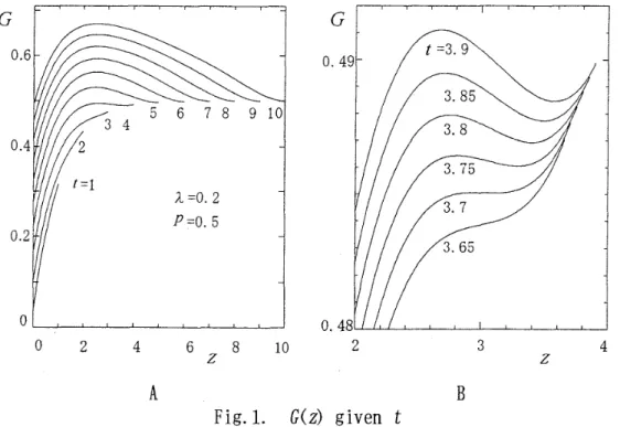
A ) varying t = 1 , 2 , --, 10. Fig. lshows the curves of G(z) given t. As shown in Fig.1-A, i f the remained search time
t i s s h o r t , G(z) i s a s t r i c t l y i n c r e a s i n g f u n c t i o n of z i n 0 5 z 5 t (see t h e curves of t = 1 . 2 and 3). In t h i s case, z* which maximizes G(z) in 0 i z i. t i s obviously a t the upper boundary; z* = t. I f t i n c r e a s e s more, G(z) has a local maximum a t z which s a t i s f i e s G'(z) = 0 ; Eq. (8). This time t is t o o = 3.75 f o r
the case of Fig. 1. Fig. 1-B shows the magnified G(z) a t the neighborhood of t o o . As shown i n Fig.1-B, G(zO) i s not maximum g l o b a l l y in 3.75< t
<
3.85; the global maximum i s s t i l l given a t the upper boundary; z* = t. The search time increases more, the ( l a r g e s t ) local maximum G(zO) grows up rapidly and z* is s h i f t e d t o the ( l a r g e s t ) l o c a l maximum p o i n t z O from t h e upper boundary a s seen i n the case of t 2 3.85 i n Fig. l - B . We have to = 3.85 f o r the case of Fig. l.Fig. 1. G(z) given t
Properties of G(z) i l l u s t r a t e d i n Fig. l a r e summarized a s follows.
[ Corol lary 1-2 l Suppose ph(0)
>
A , then G(z) has the n e x t properties.(1). G(z) is increasing in the neighborhood o f z = 0, i. e. G' (0)
>
0 f o r any t, (2). Suppose t h a t there e x i s t a p o s i t i v e t o o and t o defined by Eqs. (9) and (10).Then, if 0 S t
<
t o o , G(z) i s strictly increasing i n z c [O, tl, and if t o o S t<
t o , G(z) h a s a t l e a s t a l o c a l maximum a t z given by Eq. (8) (hence, t h e r e e x i s t s zO). If to S t, the global maximum o f G(z) is obtained a t zO.(3). If G(z) has a l o c a l siaxiam, G(z) a l s o h a s a local minimum. D
(Proof)
(1). G' (0)
>
0 i s derived from Eq. ( 6 ) by the assumption of Corollary; ph(0) > A . (2). From t h e assurnpt ion; 3 to O>
0 and t h e d e f i n i t i o n of t o o given by Eq. (g), wecan conclude G' (z)
>
0 and G(z) i s s t r i c t l y increasing in z [O, t] ; 0 i. t<
too. I f too 5 t<
t o , there e x i s t s a t l e a s t a local maximum G(z) by the d e f i n i t i o n of t o o a t z ( t ) given by Eq.(8). However, G(zO) is not the global maximum from the d e f i n i t i o n of to given by Eq (10). I f t>
t o G b O ) 2 G(t) is obvious from thedefinition of t o .
(3). If t
>
t o o 7 G(z) has a local maximum and<
0 in zO<
z<
zO+Az. However, since G 1 ( t ) = ph(t) 2 0 for the boundary t from Lemma 1-(21, G'(z) changes its sign from - to t in ( z O , tl at least once, and hence, G(z) has a local minimumin this interval, (q.e.d.)
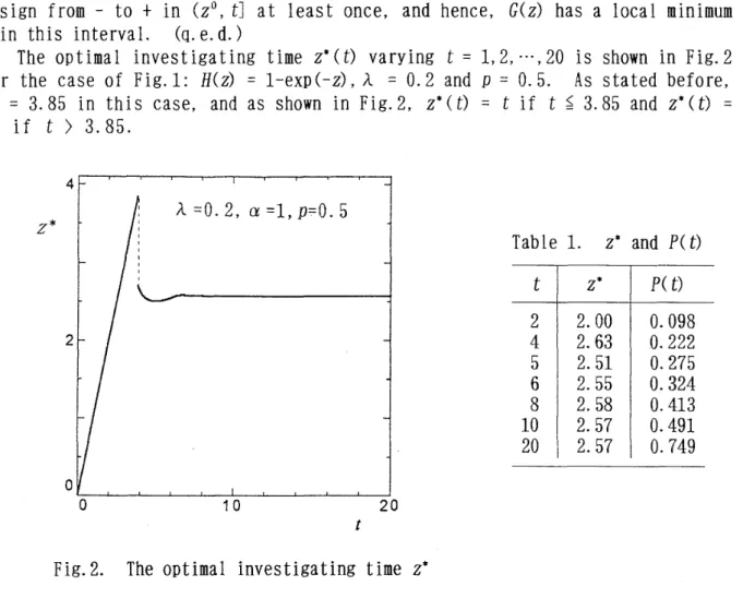
The optimal investigating time z * ( t ) varying t = 1,2, - - - , 20 is shown in Fig.2
for the case of Fig. l : H(z) = l-exp(-z), A = 0 . 2 and D = 0.5. As stated before, t o = 3.85 in this case, and as shown in Fig. 2, z* ( t ) = t if t 5 3.85 and z* ( t ) =
Table 1. z* and P( t)
Fig. 2. The optimal investigating time z*
In Fig.2, it should be noted that z * ( t ) is constant for large t. This property is presented by the next theorem.
[ Theorem 2
1
The optimal inves t i g a ting time z* converges to a constant value when the search time i s s u f f i c i e n t l y long: t à t o . U(Proof) We assume t
>
t¡ Substituting Eqs. (2) and ( 3 ) into the r. h. S. of Eq. ( 8 ) ,we have the next equation for sufficiently large t and zO à t.
The last equation is derived by substituting the next approximation for t à to and
zO ((t into the numerator of the r. h. S of the first equation.
P(t-2z0) = P( t-zO) - P' ( t - z O ) z0
Therefore, Eq. ( 8 ) becomes P ~ W / ( l - p H ( z O ) ) = A p { H W - z O h ( z O ) 1 for large t.
Since this equation does not depend on t, the solution zO of this equation also does not depend on t and becomes constant approximately if t is sufficiently
Optimal Investigating Search
From the proof of Theorem 2 , the next corollary is presented.
Corollary2-11 I f H ( z ) i s a s t r i c t l y c o n c a v e f u n c t i o n o f z w i t h h ( 0 ) > 0 and the marginal investigation rate phCz) /(l-pH(z)) i s a s t r i c t l y decreasing func- tion of z, an approximation o f zo ( t ) for t
>
t o i s given b y the unique solution zo of the next equation:(Proof) The l. h. S. of Eq. ( 1 2 ) is a strictly decreasing function of z from the
assumption of the corollary and the r. h. S. is strictly increasing by the concavity
of H(z) ; h' ( z )
<
0 . The value of the l. h. S. at z = 0 is larger than the r. h. S.since h(0)
>
0. Therefore, Eq. (12) has always a unique solution zO at which G' ( 0 )changes its sign
+
to -, and zo gives an approximation of the optimal. (q.e.d.) As mentioned later in Section 4, the solution given by E q . ( 1 2 ) is a fairly good approximation of 2%) for t>
t o . As for z o ( t ) , the next corollary isobtained.
[ Corollary 2-2
l
The approximate value z0 ( t ) for t )) to given b y Eq. (12) i s a decreasing function of A . D(Proof) Eq. (12) is rearranged as A = { . h W / ( l - p H ( z O ) ) l [ l / ( H ( z O ) - z O h ( z O ) ) l .
In the r.h.s. of this equation, the term in the first bracket is a decreasing function of zO from the assumption of Corollary 2-1 and the term in the second bracket is proved to be also a decreasing function by using the concavity of H(zo).
Hence, A is a decreasing function of zO. Therefore, if A increases, zo given by this equation is decreases. (q. e. d. )
The main properties of z * ( t ) have been elucidated by the theorems mentioned above. Here, we proceed to study the optimal investigating time Z i * ( t ) in environment
of multiple contacts classes.
3.2. Optimal plan for multiple contacts classes
In this paragraph, the case of multiple contact classes is considered. The contacts are classified into n classes and the reliability of the i-class contact
is denoted by P i , l > p i > p 2 > * - . > ~ n > 0 . Here, we define Z i O ( t ) and t i O as follows. z i O ( t ) : the value of z which gives the largest local maximum of Gi(z) in 0
<
z<
t for the i-class contact.t i O = min { t l
We have the next Theorem 3
l
(1). z i O ( t ) i s a solution o f the equation:
(2). We have
that i s , ~ i * ( t ) i s one o f {O, t, Z i 0 ( t ) } .
(3). I f the search time t i s shorter than t i O ; t
<
ti \ then zi * ( t ) = t.3 02 K. lida & R. Hohzaki & T. Kaiho
(Proof)
(1). Eq.(13) is derived from Gi'(~i(t)) = 0. Since ziO(t) gives the largest local maximum by the definition, i t satisfies this equation.
(2). The optimal zi*(t) is one of the boundary points (zj*(t) = 0 or t) or the largest local maximum point zi0(t), and therefore, Eq. (14) is obvious.
(3). Since Gi(ziO(t))
<
~ i J f i ( t ) for t<
t i O by the definition of t i o ~i*(t) iseither Zi*(t) = 0 or ~i * (t) = t by Eq. (14). Here, we assume Zi* (t) = 0 for some t i O , then there exists a time to = mimi t i O for which ~i*(t) = 0 for all i in
t
<
to. Hence, we have P(t) = 0 for all t<
to since Gi(zi*(t)) = P(t) andP'(t) = 0 by Eqs.(2) and (3). This contradicts the definition of the optimal
Zi*(t). Hence, ~ i * ( t ) = t in t < t i O is concluded.
(4). Differentiating Eq. (2) with respect to ~i(t), we have
ihi ( 2 )
Gi'
(zi
(t)) )(S) 0 2 l!piHi (z) )(S) l-~(t-~,) P' ( t-~i)(The signs
>
and S are appl ied in same order. )Here, we assume Ineq. (15). We have Gi ' (0)
>
0 from Eq. (161, and to neglect the i-class contact is not optimal since the investigation is effective to increase the detection probability. Hence, Zi*(t)>
0 if Ineq.(15) holds. (q.e.d.) In the case of mu1 tiple contact classes, some ineffective contacts are neglected in the investigation in t>
to. In Section 4, we shall show a numerical example in which the contact with low reliability is neglected. The next corollary is directly derived from Theorems 3421, (3) and the definition of tiO.[Corollary3-11 Suppose thereexists t i O . I f 0 < t i tiO, Zi*(t) = t. If
t ) tiO and Gi(zi0(t))
>
PO),
then Zi*(t) = ziO and if t>
tiO and Gi(ZiO(t))5
PO),
then ~i*(t) = 0. DThe meaning of this corollary will be discussed in Section 5.
The relations between the optimal investigating time of the i-class contact and the (it1)-class contact are presented by the next theorem.
[ Theorem 4 l
(l). If pihi(Z) 2 pi+ihi+i(z) in 0 5 z 5 t, we have the relation; tiO 2 ti+iO.
(2). If pihi(Z) 2 pi+ihi+i(z) in 0 2 z 5 t, the optimal investigating times for
the contacts i and it1 classes have the relation; ~ i * ( t ) 2 ~i+i*(t). D (Proof)
(1). We define A G M = Gi (2)-Gi+i (z), then we can easily confirm that AG(z) is
an increasing function of z if pihi(z) 2 pi+ihi+i(z) in z â ‚ ¬ [ tl. Since zi* (t) 2 t for all t and any i, we have AG( t) 2 AG(zi*( t)), and therefore,
Gi(t) - Gi(zi*(t)) 2 Gi+i(t) - Gi+i(Zi*(t)).
From the above, we have the next inequality since Gi+i(~i+i*(t)) 2 Gi+i(zi*(t)). Here, to prove Theorem by the reductive absurdity, we suppose t i O
<
t i + i O andconsider t such as t i O
<
t<
ti+l'.
Then, the r. h. S. of the above inequal i ty is zero since ~i*(t)<
t and Zi+i*(t) = t from Corollary 3-1, and therefore, wehave Gi(t)
>
Gi (Zi*(0).
This contradicts the definition of the optimal zi*(t).Therefore, tiO 2 ti+iO is concluded.
Optimal In vestjgatin~ Search 303
From the above, we have
On the other hand, AG(z) = Gi(~)-Gi+i(~) is a strictly increasing function of z if pihi(z) 2 pi+ihi+i(z) as mentioned above. Here, we assume ~i*(t)
<
Zi+i*(t), then since AG(z) is the increasing function of z, AG(zi*(t))<
AG(zi+i* (t)), we have the relation ;This inequality contradicts Ineq. (17), and therefore, Zi*(t) 2 Zi+i*(t) is concluded. (a. e. d. )
FCorollary4-1
1
If thefunctionHi(z) is common toall contacts;Hi(z) = H(z)for all i, wehave relations; t i O 2 t i + i o andzi*(t) 2 Zi+i*(t). D
(Proof) If Hi(Z) is common to all contact, pihi(Z) 2 pi+lhi+i(Z) in all z, 0 5 z
5 t, is obvious from the definition of pi, and therefore, Corollary is established by Theorem 4.
(a.
e. d.)[ Theorem 5
l
Suppose the marginal investigation rate ; pihi (z) /(l-piHi (2)) is a decreasing function of z. If A (= increases, z-:*(t) for t>
t i O decreases. D(Proof) Let fi = A i/A, where A (= E iA i) is the rate of any contact and fi
is the conditional probability of the i-class contact when a contact is gained. Rewriting EQ. (3) by using A and fi, we have P'U) = A S ifi{Gi(zi*(t))-P(t)}, hence, P' (t) (obviously P' ( t) 2 0 and Gi (Zi * ( t)) 2 P( t)) increases as A increases. Since the r. h. S. of Eq. (13) increases as A increases, and the solution zi * (t) of Eq. (13) decreases because the l. h. S. of Eq. (13) is strictly decreasing function of ~ i (t) * by the assumption of Theorem. (q. e. d. )
4. Numerical Examples
In this section, assuming the exponential investigating function ; &(z) =
l-exp(- a iz), we analyze several numerical examples to see the sensitivity of the system parameters to the optimal investigating plan. Here, taking the mean investigating time of Contact 1 as the unit time, we set a l = 1. For the sake
of convenience for the numerical analysis of this section, we define the contact rate A = S i A i and the conditional probability of the i-class contact fi = A -:/A,
then obviously A i = f i A . Hereafter, we set the primary case, Case 1, and then
varying system parameters in Cases 2, 3 and 4, we evaluate the optimal investigat- ing plan to see the sensitivities of each parameter. Here, we set the parameters of Case 1 as
Case 1 : n = 3, {pi} = {0.9, 0.5, 0.11,
a i = l for all i, A = Â £ i A = 0.2,
{fi} = { A i/A = {1/3,1/3,1/3}.
The optimal investigating plan of Case 1 is calculated discretely by every At =
0.01 using Eqs. (2), (3), (4) and (5). The solutions, zi * ( t) and P( t) are presented
in Table 2 and ~ i
(0,
* i=l, 2,3, are visualized in Fig. 3. As seen in Fig. 3, theproperties described in Corollary 3-1 ; if t S t i O , ~i*(t) =t, and if t
>
tiO, zi*(t) = ziO, Corollary 4-1 ; tiO 2 ti+i¡ and Zi*(t) 2 ~i+i*(t), are shown clearly.Next, to examine the sensitivity of the rate of contacts A = S iA i , A is varied from A = 0.2 in Case 1 to A = 0.1 in Case 2, whereas the other parameters
K. lid8 & R. Hohzaki & T. Kaiho
Fig. 3. The optimal plan of Case 1 are kept the same as Case 1 :
Case 2 : /I = 0.1.
Furthermore, to see the sensitivity of A i keeping constant /I = 0.2, we evaluate
Case 3 varying fi from { f i
l
= {1/3,1/3,1/3l in Case 1 toCase 3 : { fi 1 = {O. 8, 0.1, 0. l}.
The optimal investigating plans of Cases 2 and 3 are evaluated and shown in Table 3 and are visualized in Figs. 4 and 5, respectively. BY comparing Fig. 4 (Case 2) with Fig. 3 (Case l), we can see that the optimal investigating time increases when /I decreases as stated in Theorem 5. In Fig. 5 (Case 3), it should be noted that Contact 3 is neglected in the optimal investigating plan for t
>
tsO. This corresponds to the case: t>
tiO and Gi (ziO (t)) 5 P(t)l
in Corollary 3-1, and then Zi*(t) = 0.Table 3 2,-*(t) and P(t) of Cases 2 and 3
Optimal Investigating Search 305
Fig. 4. The optimal plan of Case 2 Fig. 5. The optimal plan of Case 3 To examine the extreme value of Gi(~i(t))
in
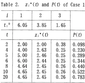
detail for Case 3, we evaluate the marginal investigation rate ; k A i ( ~ i (t))/{l-piffi (zi ( t ) ) 1 (referred to Ai-curve)and the marginal detect ion rate ; P' ( t-zi ( t) /{!-P( t-Z, ( t) ) 1 (referred to P'-curve) at t = 2,5.10 and show them in Fig. 6. From Eq. (16), we can see that Gi ' (z) > ( S ) 0 2 A,-curve > ( S ) P'-curve. As shown in Fig. 6-A. if t = 10. hi-curves, i = 1,2,
have two intersections with P'-curve. We can easily confirm by Ea. (16) that the smaller Zi of the intersection corresponds to the local maximum (the optimal zi*)
and the larger one does the local minimum. On the other hand, the h-curve has
J
0 5 10 0 5
J
10 0 5 1010 5 0 10 5 0 10 5 0
-Ã z t-z + -*Â z t-z + - + z t-z +
306 K. Iida & R. Hohzaki & T. Kaiho
only one intersection with P'-curve at z = 10 and it gives the local minimum.
Hence if G3 (0)
>
G3 (t), the global maximum is given by G i (0). In this case, we have G3(0) = P(t) = 0.710 and G3(t) = ~3^3(t) = 0.1 at t = 10 and ~3*(t)= 0 is confirmed. Next let' s consider the case of t = 5 in Fig. 6-B. In this case, hi- curve is always larger than P'-curve in z e 10, t] and G A z )>
0 in this interval, hence, maxoazs Gi (z*) = G&), namely, zi* (5) = 5. As for hi-curve, i = 2,3,the intersections of hi-curve with P'-curve are same as the case of t = 10 and m a x o ~ ~ ~ ~ G2(z) is the local maximum and maxoszsit GAz) = G3(0) as stated above. Next, we examine the case of t = 2 (Fig. 6-0. In this case, hi-curves, i = 1,2, are always larger than P'-curve in z c [O, tl and then maxoazst G i b ) = Gi(t), i =
1,2, and h3-curve is the same as Fig. 6-A.
Next, we examine Case 4 in which the investigating rates a i are changed from
a i = 1, i = 1,2,3, in Case 1 to
Case 4 : a i = 1 and a2 = a 3 = 0.5.
In this case, the Contacts 2 and 3 are time-consuming to investigate compared with Contact 1 (it takes twice longer investigating time of Contacts 2, 3 than that of Contact 1 on the average). The optimal investigating plan is shown in Table 4 and Fig. 7. By Comparing Fig. 7 (Case 4) with Fig. 3 (Case l), we can see that Contact 3
is neglected in t
>
ts0 in Case 4, and Contacts 1 and 2 are investigated thorough-ly, namely, the investigating time for these contacts are prolonged in Case 4.
The results of Cases 3 and 4 seem to be instructive. The assertions of these Cases are stated as follows. The contacts with poor reliability or low efficiency should be neglected and the investigating effort should be concentrated to the contact with high reliability and efficiency if there is plenty of search time remained, and if the remained time is short, all contacts should be investigated until the end of the search. This assertion may be reasonable intuitively and Theorems are very useful to give a explicit quantitative bases for the decision of the optimal investigating search plan.
Final ly, assuming single contact class and the exponential investigating func- tion H(z) = l-exp(- a z), we examine the accuracy of the approximation zO given
. . . ,
i=O. 2, /=1/3 Table 4. 2,-*(t) and P(t) of Case 4
-
- pi=O. 9, a 1=1
Optimal Investigating Search 307
by Eq. (12) for t
>
t i o . Substituting H(z) into Eq. (12), we have the next equa- t ion ofzO.
Applying the Newton method to the above equation, we obtain the solution zO = 2.55
for the example given in Section 3.1 ; A = 0.2, ec = 1, p = 0.5. In this case,
the optimal investigating time z* (20) = 2.57 is given as shown in Table 1. The
absolute error of zO is 0.02 and the relative error is only 0.8 %. This accuracy of the approximation may be sat isfactory for the use of practical applications. However, as mentioned before, the approximation zO given by Eq. (12) is derived
by assuming the single contact class. If we apply Eq. (12) to the case of the mu1 tiple contacts classes, the approximation is not sufficient; we must consider other approximations than this for the mu1 t iple contacts classes.
5. Discussions
In this section, we elucidate the meaning of the conditions of the optimal investigating plan and discuss the differences between the optimal plan obtained above and that of the previous studies.
5.1. Interpretation of the conditions for the optimal plan
(l). The assertions of Corollary 1-1 or 3-1 is stated as follows ; if the remained search time is short, i t should be used exhaustively to investigate the contact on his hand, and if plenty of search time is remained, the investigation should be stopped at some appropriate time. This assertion seems to be reasonable since the searcher cannot expect to gain a new contact in the broad search if the remained time is short, and then he should not stop the investigation to the contact on his hand. On the contrary, if the remained time is long enough to detect a new contact, he should stop the investigation of the suspicious contact and return to the broad search for new contacts. When the optimal investigating search is stopped at ziO (t), the optimal condition of z* given by Eq. (13) is elucidated as follows. The l. h. S. of Eq. (13) is the conditional investigating
probability of the contact being examined in unit time at z* given that i t has been investigated until z* unsuccessfully (called the marginal investigation rate). On the other hand, the r.h.s. of Eq.(13) is the conditional detection probability in unit time when the searcher stops the investigation at z* and return to the broad search (called the marginal detection rate of the broad search). The optimal stopping time z* is the balance point of the both marginal values mentioned above. Such property is reasonable for the optimal conditions of the investigating search.
(2).
As
stated in Corollary 2-2 and Theorem 5, if A increases, z* (t) for t>
to decreases. This property seems to be natural since we can expect to contact frequently when A is large, and then the searcher does not necessary to stick to a contact, and therefore, he should stop the investigation early.(3). In the case of multiple contacts classes, if the search time t
<
t i O , z i * ( t )= t for any i as stated in Theorem 3-(3), and if P i is small enough, zi*(t) = 0 for
t
>
t i O as shown in the examples; Cases 3 and 4in
Section 4. This property isdeduced from the similar reason discussed above in (l), namely, if the remained time is short, since the searcher cannot expect to gain a new contact in the broad
308 K. Iida & R. Hohzaki & T. Kaiho
search, he should continue his investigation for any contact even if its relia- bility is low, on the contrary, if the remained time is long enough to detect a new contact, he should neglect the contact with low reliability and return to
the broad search for new contacts.
From the view point of real world applications, we may be able to approx- imate the optimal plan by such a plan controlled by two values t i o and Zi that
zi*(t) = tfor t < t,¡andzi*(t = z i f o r a n y t 2 t i V f it isinvestigated. The
validity of this approximation is expected from the numerical examples shown in Sect ion 3.
(4). As for the time t i o if pihi(t)
>
pj+ihi+i(t), we have the relation; tiO2 ti+i as stated in Theorem 4 4 , and the optimal investigating time has the
relation ; ~i*(t) 2 Zi+i*(t) by Theorem 442). These properties are the same as mentioned above in (1) and ( 3 ) ; the contact with high reliability should be investi- gat ed thorough l y.
5.2. Relations to the optimal plans studied previously
As stated in Section 1, Kisi [31 presented a model of the similar investi- gating search to our model. Assuming single contact class, a large number of targets and Poisson arrival of the contact in the broad search, he formulated the model with the criterion of the expected number of the target detected in time T. He gave the equation of the optimal investigating time and showed several numerical examples. Let E(t) be the maximum expected number of detected target when time t remains. The necessary condition of the optimal investigating t ime is given by
Assuming H(z) = l-exp (- o! z) in Eq. (191, Kisi derived the next equation of z* ( t)
for a sufficiently large t.
Eqs. (19) and (20) correspond to Eqs. (8) and (18) in our model. Comparing the r. h. S.
of Eq. (18) with Eq. (20), we can see that the optimal investigating time zO of our model given by Eq. (18) is larger than that of Kisi' S model given by Eq. (20).
Iida 121 studied the optimal investigating search under assumptions of mu1 ti- pie contact classes and unrestricted search time with the criterion of expected time to detection. Let ET be the expected time to detection by the optimal plan. The equation of the optimal investigating time ~ i *is given by
In this case, the optimal investigating plan such as zi*(t) = t stated in Corol- laries 1-1 and 3-1 does not exist since the search time is not restricted.
6. Conc lud ing Remarks
In this paper, we consider a two-stage search consisting of the broad search and the investigating search for false contacts caused by system noise. We study the optimal stopping time of the investigating search maximizing the detection probability of the target until the end of the search. We derive the
Optimal Investigating Search 309
conditions of the optimal investigating search plan and give clear interpreta- tions for the conditions. Furthermore, by using the conditions, we elucidate the structure of the optimal plan and explain its behavior when the system parameters are varied.
Acknowledgment S
The authors would like to express their sincere thanks to anonymous referees for their useful comments and suggest ions to refine this paper.
References
[l] Dobbie, J. M. , "Some Search Problems with False Contacts, " Operations Research, 21 (1973), pp. 907-925.
[21 Iida, K., "Optimal Stopping of a Contact Investigation, " Mathematica Japonica, 34 (1989), pp. 169-190.
[31 Kisi, T., "Optimal Stopping of the Investigating Search," in Search Theory and Applications, NATO Conference Series 1-8, pp.255-260, Plenum Press, N.Y., 1979.
[41 Koopman, B.O. Search and Screening, 2nd ed., Ch.3, pp.71-74, Pergamon Press, N.Y., 1980.
[51 Stone, L. D. , Theory of Optimal Search, 2nd ed., Ch. 6, pp. 136-178, Mil. Appl. Sec. of ORSA, Ket ron Inc. , Va. , 1981.
[61 Stone, L. D. and Stanshine, J. A. , "Optimal Search Using Uninterrupted Contact Investigation, " SIAM. 1. Awl. Math. , 20 (1971). pp. 241-263.
[71 Stone, L. D., Stanshine, J. A. and Persinger, C. A. , "Optimal Search in the Presence of Poi sson-Dist ributed Fa1 se Target, " SIAM. J. Appl. Ma th. , 23 (1972),
pp. 2-27.
[81 Washburn, A. R. , Search and Detection, Â 2.2, pp. 2.4-2.8, Mil. Appl. Sec. of ORSA, Ketron Inc., Va. , 1981.
Koj i IIDA : Department of Applied Physics, National Defense Academy,
Hashi rimizu 1-10-20, Yokosuka, 239, Japan.